Only need help answering question 7,8, and 9
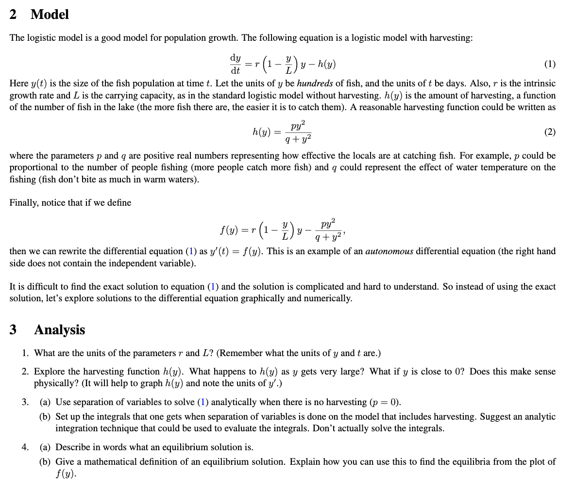
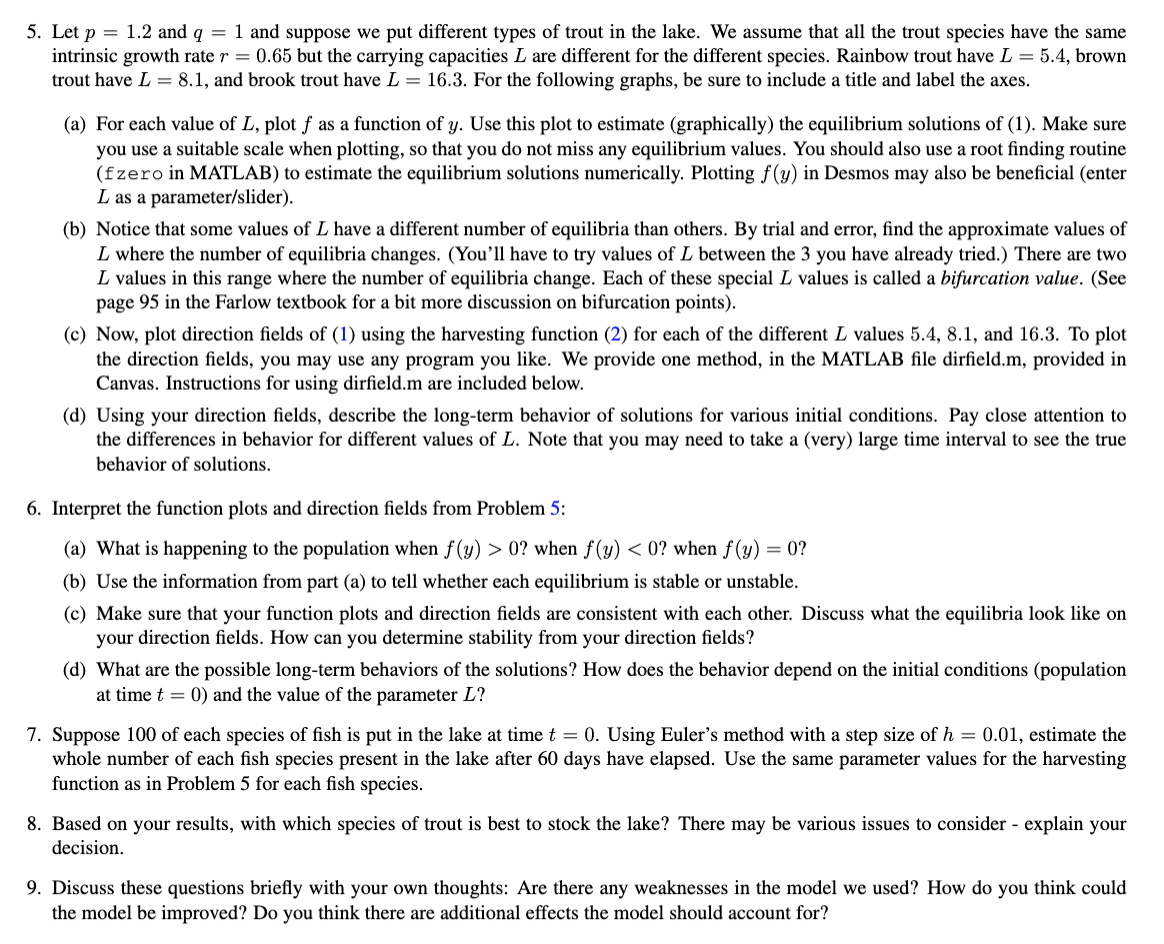
2 Model The logistic model is a good model for population growth. The following equation is a logistic model with harvesting: %=r(l_%)yhtw (1) Here y(t) is the size of the sh population at time t. Let the units of y be hundreds of sh, and the units of t be days. Also, 1' is the intrinsic growth rate and L is the carrying capacity, as in the standard logstic model without harvesting. My) is the amount of harvesting, a function of the number of sh in the lake (the more sh there are, the easier it is to catch them). A reasonable harvesting function could be written as 2 37.1} h 3; = (2) { ) q + 92 where the parameters p and q are positive real numbers representing how effective the locals are at catching sh. For example, p could be proportional to the number of people shing (more people catch more sh) and q could represent the effect of water temperature on the shing (sh don't bite as much in warm waters). Finally, notice that if we dene 2 f(y)=r(l-%)yq:yy2, then we can rewrite the differential equation (1) as y'(t) = f (y). This is an example of an autonomous differential equation (the right hand side does not contain the independent variable). It is difcult to nd the exact solution to equation (1) and the solution is complicated and hard to understand. So instead of using the exact solution, let's explore solutions to the differential equation graphically and numerically. 3 Analysis 1. What are the units of the parameters r and L? (Remember what the units of y and t are.) 2. Explore the harvesting function h(y). What happens to h(y) as 3; gets very large? What if y is close to 0? Does this make sense physically? (It will help to graph My) and note the units of y'.) 3. (a) Use separation of variables to solve (1) analytically when there is no harvesting (p = 0). (b) Set up the integrals that one gets when separation of variables is done on the model that includes harvesting. Suggest an analytic integration technique that could be used to evaluate the integrals. Don't actually solve the integrals. 4. (a) Describe in words what an equilibrium solution is. (b) Give a mathematical denition of an equilibrium solution. Explain how you can use this to nd the equilibria from the plot of y)- 5. Let p = 1.2 and q = 1 and suppose we put different types of trout in the lake. We assume that all the trout species have the same intrinsic growth rate r = 0.65 but the carrying capacities L are different for the di'erent species. Rainbow trout have L = 5.4, brown trout have L = 8.1, and brook trout have L = 16.3. For the following graphs. be sure to include a title and label the axes. (a) For each value of L, plot f as a function of y. Use this plot to estimate (graphically) the equilibrium solutions of (1). Make sure you use a suitable scale when plotting, so that you do not miss any equilibrium values. You should also use a root nding routine (f zero in MATLAB) to estimate the equilibrium solutions numerically. Plotting f (y) in Desmos may also be benecial (enter L as a parameterlslider). (b) Notice that some values of L have a different number of equilibria than others. By trial and error, find the approximate values of L where the number of equilibria changes. (You'll have to try values of L between the 3 you have already tried.) There are two L values in this range where the number of equilibria change. Each of these special L values is called a bifurcation value. (See page 95 in the Farlow textbook for a bit more discussion on bifurcation points). (c) Now, plot direction elds of (1) using the harvesting function (2) for each of the different L values 5.4, 8.1, and 16.3. To plot the direction elds, you may use any program you like. We provide one method, in the MATLAB le direldm, provided in Canvas. Instructions for using direld.m are included below. (d) Using your direction elds, describe the long-term behavior of solutions for various initial conditions. Pay close attention to the differences in behavior for different values of L. Note that you may need to take a (very) large time interval to see the true behavior of solutions. 6. Interpret the function plots and direction elds from Problem 5: (a) What is happening to the population when y) > 0'? when f (y)