Original code to cut and paste

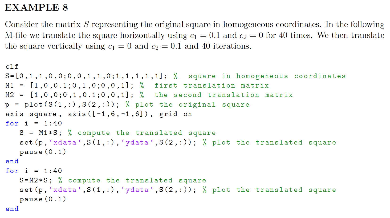
clf

S=[0 ,1 ,1 ,0 ,0;0 ,0 ,1 ,1 ,0;1 ,1 ,1 ,1 ,1]; % square in homogeneous coordinates

M1 = [1 ,0 ,0.1;0 ,1 ,0;0 ,0 ,1]; % first translation matrix

M2 = [1 ,0 ,0;0 ,1 ,0.1;0 ,0 ,1]; % the second translation matrix

p = plot (S(1 ,:) ,S (2 ,:)); % plot the original square

axis square , axis ([ -1 ,6 , -1 ,6]) , grid on

for i = 1:40

S = M1*S; % compute the translated square

set(p,'xdata ',S(1 ,:) , 'ydata ',S (2 ,:)); % plot the translated square

pause (0.1)

end

for i = 1:40

S=M2*S; % compute the translated square

set(p,'xdata ',S(1 ,:) , 'ydata ',S (2 ,:)); % plot the translated square

pause (0.1)

end

EXAMPLE 8 Consider the matrix S representing the original square in homogeneous coordinates. In the following M-file we translate the square horizontally using ci = 0.1 and c2 = 0 for 40 times. We then translate the square vertically using ci = 0 and c2 = 0.1 and 40 iterations. 11 clf S=[C square in homogeneous coordinates M1 = [1,0,0.1;0,1,0;0,0,1]; % first translation matrix M2 = (1,0,0;0,1,0.1;0,0,1); % the second translation matrix p = plot(S (1,:), S (2,:)); % plot the original square axis square, axis ([-1,6,-1,6]), grid on for i = 1:40 S = M1*S; % compute the translated square set(p, 'xdata',S(1,:), 'ydata',S(2,:)); % plot the translated square pause (0.1) end for i = 1:40 S=M2*S; % compute the translated square set(p, 'xdata',S(1,:), 'ydata', S (2,:)); % plot the translated square pause (0.1) end 6. Modify the M-file in EXAMPLE 8 adding translations that bring the square to its original position using 40 iterations and a single additional for loop. Include the M-file (for a total of three loops) You do not need to include the figure. EXAMPLE 8 Consider the matrix S representing the original square in homogeneous coordinates. In the following M-file we translate the square horizontally using ci = 0.1 and c2 = 0 for 40 times. We then translate the square vertically using ci = 0 and c2 = 0.1 and 40 iterations. 11 clf S=[C square in homogeneous coordinates M1 = [1,0,0.1;0,1,0;0,0,1]; % first translation matrix M2 = (1,0,0;0,1,0.1;0,0,1); % the second translation matrix p = plot(S (1,:), S (2,:)); % plot the original square axis square, axis ([-1,6,-1,6]), grid on for i = 1:40 S = M1*S; % compute the translated square set(p, 'xdata',S(1,:), 'ydata',S(2,:)); % plot the translated square pause (0.1) end for i = 1:40 S=M2*S; % compute the translated square set(p, 'xdata',S(1,:), 'ydata', S (2,:)); % plot the translated square pause (0.1) end 6. Modify the M-file in EXAMPLE 8 adding translations that bring the square to its original position using 40 iterations and a single additional for loop. Include the M-file (for a total of three loops) You do not need to include the figure