other lines remains unchanged. Calculate the optimal dispatch and the nodal prices for these conditions. $[$Hint: the optimal solution involves a redispatch of generating units at all three buses$]$

$6\mathrm{.}10$ Consider the two$-$bus power system of Problem $6\mathrm{.}2.$ Given that $\backslash ($ K$=$R $/$ V$^\{2\}=\backslash )\backslash (0\mathrm{.}0001\backslash$mathrm$\{$MW$\}^\{-1\}\backslash )$ for the line connecting buses A and B and that there is no limit on the capacity of this line, calculate the value of the flow that minimizes the total variable cost of production. Assuming that a competitive electricity market operates at both buses, calculate the nodal marginal prices and the merchandising surplus. $[$Hint: use a spreadsheet$].$

$6\mathrm{.}11$ Repeat Problem $6\mathrm{.}10$ for several values of $\backslash ($ K $\backslash )$ ranging from $0$ to $0\mathrm{.}0005.$ Plot the optimal flow and the losses in the line, as well as the marginal cost of electrical energy at both buses. Discuss your results.

$6\mathrm{.}12$ Using the linearized mathematical formulation $($dc power flow approximation$),$ calculate the nodal prices and the marginal cost of the inequality constraint for the optimal redispatch that you obtained in Problem $6\mathrm{.}7.$ Check that your results are identical to those that you obtained in Problem $6\mathrm{.}8.$ Use bus $3$ as the slack bus.

$6\mathrm{.}13$ Show that the choice of slack bus does not influence the nodal prices for the dc power flow approximation by repeating Problem $6\mathrm{.}12$ using bus $1$ and then bus $2$ as the slack bus.

$6\mathrm{.}14$ Using the linearized mathematical formulation $($dc power flow approximation$),$ calculate the marginal costs of the inequality constraints for the conditions of Problem $6\mathrm{.}9.$

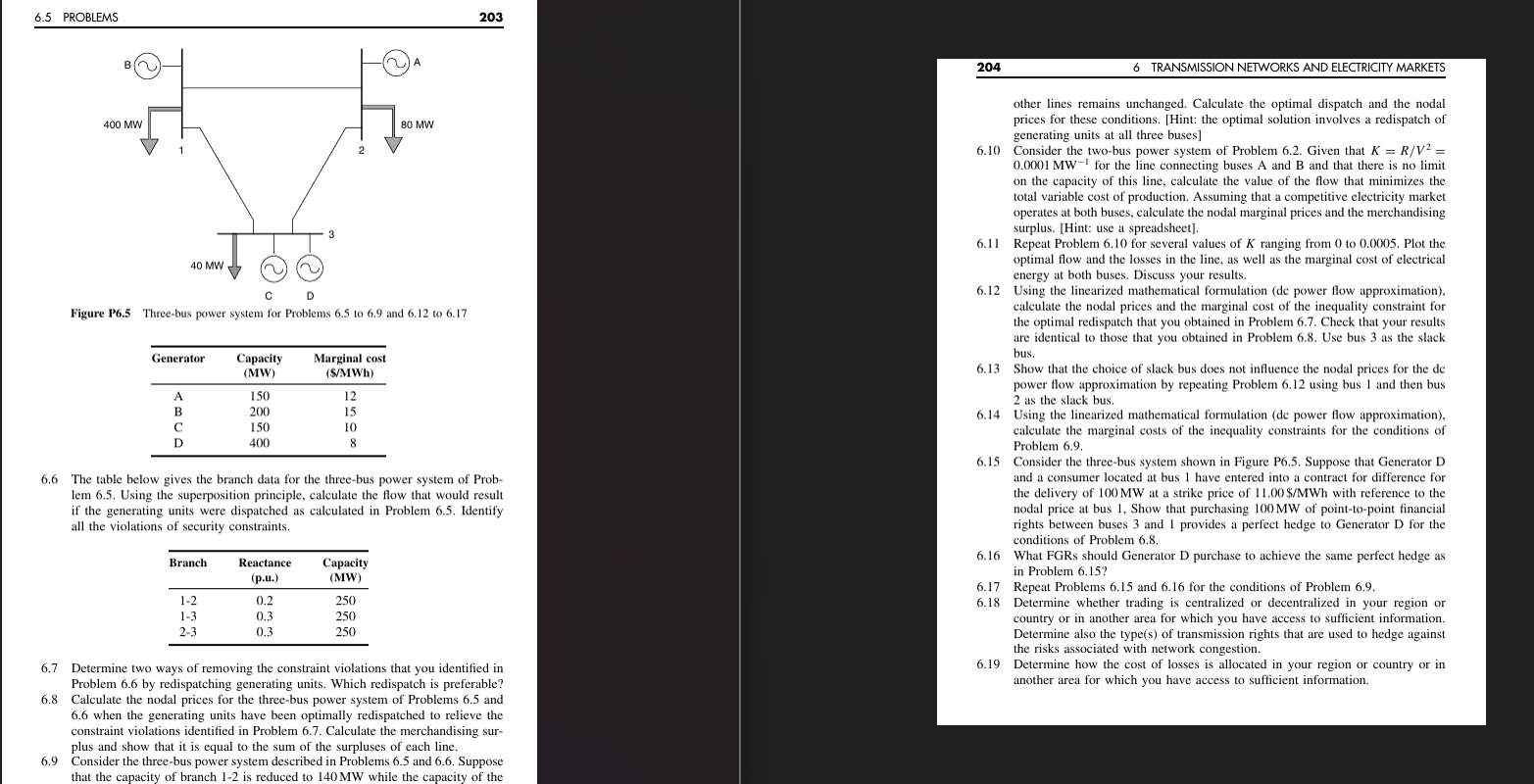
$6\mathrm{.}15$ Consider the three$-$bus system shown in Figure P$6\mathrm{.}5.$ Suppose that Generator D and a consumer located at bus $1$ have entered into a contract for difference for the delivery of $100$ MW at a strike price of $\backslash (11\mathrm{.}00\backslash$$ $/\backslash$mathrm$\{$MWh$\}\backslash )$ with reference to the nodal price at bus $1,$ Show that purchasing $100$ MW of point$-$to$-$point financial rights between buses $3$ and $1$ provides a perfect hedge to Generator D for the conditions of Problem $6\mathrm{.}8.$

$6\mathrm{.}16$ What FGRs should Generator D purchase to achieve the same perfect hedge as in Problem $6\mathrm{.}15?$

$6\mathrm{.}17$ Repeat Problems $6\mathrm{.}15$ and $6\mathrm{.}16$ for the conditions of Problem $6\mathrm{.}9.$

$6\mathrm{.}18$ Determine whether trading is centralized or decentralized in your region or country or in another area for which you have access to sufficient information. Determine also the type$($s$)$ of transmission rights that are used to hedge against the risks associated with network congestion.

$6\mathrm{.}19$ Determine how the cost of losses is allocated in your region or country or in another area for which you have access to sufficient information. Figure P$6\mathrm{.}5$ Three$-$bus power system for Problems $6\mathrm{.}5$ to $6\mathrm{.}9$ and $6\mathrm{.}12$ to $6\mathrm{.}17$

$6\mathrm{.}6$ The table below gives the branch data for the three$-$bus power system of Problem $6\mathrm{.}5.$ Using the superposition principle, calculate the flow that would result if the generating units were dispatched as calculated in Problem $6\mathrm{.}5.$ Identify all the violations of security constraints.

$6\mathrm{.}7$ Determine two ways of removing the constraint violations that you identified in Problem $6\mathrm{.}6$ by redispatching generating units. Which redispatch is preferable?

$6\mathrm{.}8$ Calculate the nodal prices for the three$-$bus power system of Problems $6\mathrm{.}5$ and $6\mathrm{.}6$ when the generating units have been optimally redispatched to relieve the constraint violations identified in Problem $6\mathrm{.}7.$ Calculate the merchandising sur$-$

other lines remains unchanged. Calculate the optimal dispatch and the nodal prices for these conditions. $[$Hint: the optimal solution involves a redispatch of generating units at all three buses$]$

$6\mathrm{.}10$ Consider the two$-$bus power system of Problem $6\mathrm{.}2.$ Given that $\backslash ($ K$=$R $/$ V$^\{2\}=\backslash )\backslash (0\mathrm{.}0001\backslash$mathrm$\{$MW$\}^\{-1\}\backslash )$ for the line connecting buses A and B and that there is no limit on the capacity of this line, calculate the value of the flow that minimizes the total variable cost of production. Assuming that a competitive electricity market operates at both buses, calculate the nodal marginal prices and the merchandising surplus. $[$Hint: use a spreadsheet$].$

$6\mathrm{.}11$ Repeat Problem $6\mathrm{.}10$ for several values of $\backslash ($ K $\backslash )$ ranging from $0$ to $0\mathrm{.}0005.$ Plot the optimal flow and the losses in the line, as well as the marginal cost of electrical energy at both buses. Discuss your results.

$6\mathrm{.}12$ Using the linearized mathematical formulation $($dc power flow approximation$),$ calculate the nodal prices and the marginal cost of the inequality constraint for the optimal redispatch that you obtained in Problem $6\mathrm{.}7.$ Check that your results are identical to those that you obtained in Problem $6\mathrm{.}8.$ Use bus $3$ as the slack bus.

$6\mathrm{.}13$ Show that the choice of slack bus does not influence the nodal prices for the dc power flow approximation by repeating Problem $6\mathrm{.}12$ using bus $1$ and then bus $2$ as the slack bus.

$6\mathrm{.}14$ Using the linearized mathematical formulation $($dc power flow approximation$),$ calculate the marginal costs of the inequality constraints for the conditions of Problem $6\mathrm{.}9.$

$6\mathrm{.}15$ Consider the three$-$bus system shown in Figure P$6\mathrm{.}5.$ Suppose that G