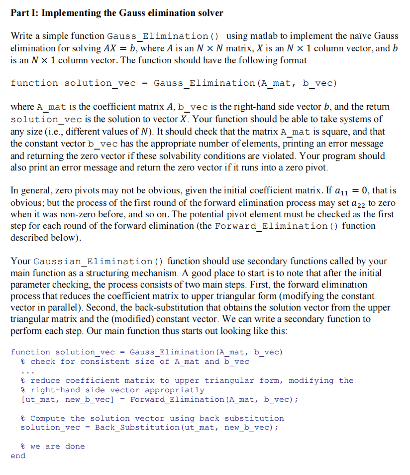
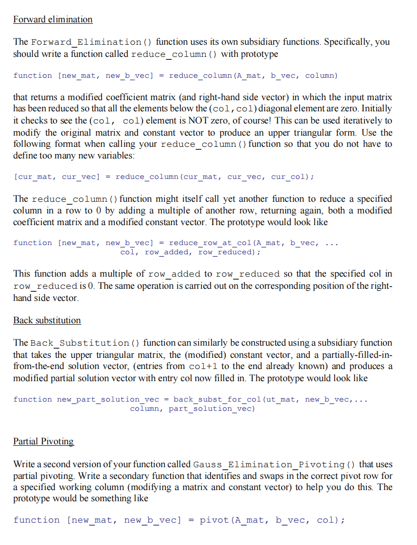
Part I: Implementing the Gauss elimination solver Write a simple function Gauss_Elimination () using matlab to implement the nave Gauss elimination for solving AX = b, where A is an N * N matrix, X is an N * 1 column vector, and b is an N * 1 column vector. The function should have the following format function solution_vec = Gauss_Elimination (A_mat, b_vec) where A_mat is the coefficient matrix A, b_vec is the right-hand side vector b, and the return solution_vec is the solution to vector X. Your function should be able to take systems of any size (i.e., different values of N). It should check that the matrix A_mat is square, and that the constant vector b_vec has the appropriate number of elements, printing an error message and returning the zero vector if these solvability conditions are violated. Your program should also print an error message and return the zero vector if it runs into a zero pivot. In general, zero pivots may not be obvious, given the initial coefficient matrix. If a11 = 0, that is obvious; but the process of the first round of the forward elimination process may set az2 to zero when it was non-zero before, and so on. The potential pivot element must be checked as the first step for each round of the forward elimination (the Forward_Elimination () function described below). Your Gaussian_Elimination () function should use secondary functions called by your main function as a structuring mechanism. A good place to start is to note that after the initial parameter checking, the process consists of two main steps. First, the forward elimination process that reduces the coefficient matrix to upper triangular form (modifying the constant vector in parallel). Second, the back-substitution that obtains the solution vector from the upper triangular matrix and the (modified) constant vector. We can write a secondary function to perform each step. Our main function thus starts out looking like this: function solution_vec = Gauss_Elimination (A_mat, b_vec) % check for consistent size of A_mat and b_vec % reduce coefficient matrix to upper triangular form, modifying the & right-hand side vector appropriatly [ut_mat, new_b_vec] = Forward_Elimination (A_mat, b_vec); & Compute the solution vector using back substitution solution_vec Back_Substitution (ut_mat, new_b_vec); % we are done end Forward elimination The Forward_Elimination () function uses its own subsidiary functions. Specifically, you should write a function called reduce_column() with prototype function [new_mat, new_b_vec] = reduce_column (A_mat, b_vec, column) that returns a modified coefficient matrix (and right-hand side vector) in which the input matrix has been reduced so that all the elements below the (col, col) diagonal element are zero. Initially it checks to see the (col, col) element is NOT zero, of course! This can be used iteratively to modify the original matrix and constant vector to produce an upper triangular form. Use the following format when calling your reduce_column() function so that you do not have to define too many new variables: [cur_mat, cur_vec] = reduce_column (cur_mat, cur_vec, cur_col); The reduce_column() function might itself call yet another function to reduce a specified column in a row to 0 by adding a multiple of another row, returning again, both a modified coefficient matrix and a modified constant vector. The prototype would look like function [new_mat, new_b_vec] = reduce_row_at_col (A_mat, b_vec, col, row_added, row_reduced); This function adds a multiple of row_added to row_reduced so that the specified col in row_reduced is 0. The same operation is carried out on the corresponding position of the right- hand side vector Back substitution The Back_Substitution () function can similarly be constructed using a subsidiary function that takes the upper triangular matrix, the (modified) constant vector, and a partially-filled-in- from-the-end solution vector, (entries from col+1 to the end already known) and produces a modified partial solution vector with entry col now filled in. The prototype would look like function new_part_solution_vec = back_subst_for_col (ut_mat, new_b_vec, ... column, part_solution_vec) Partial Pivoting Write a second version of your function called Gauss_Elimination_Pivoting () that uses partial pivoting. Write a secondary function that identifies and swaps in the correct pivot row for a specified working column (modifying a matrix and constant vector) to help you do this. The prototype would be something like function [new_mat, new_b_vec] = pivot (A_mat, b_vec, col); Write a function to swap a specified pair of rows (modifying both the coefficient matrix and constant vector) with prototype function [new_mat, new_vec] = = swap_rows (mat, vec, rowl, row2)