Please adapt the given MATLAB script to solve the problem


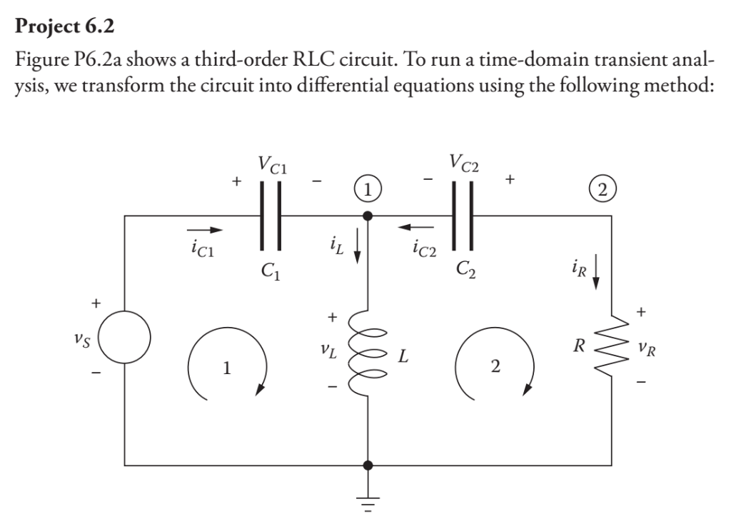
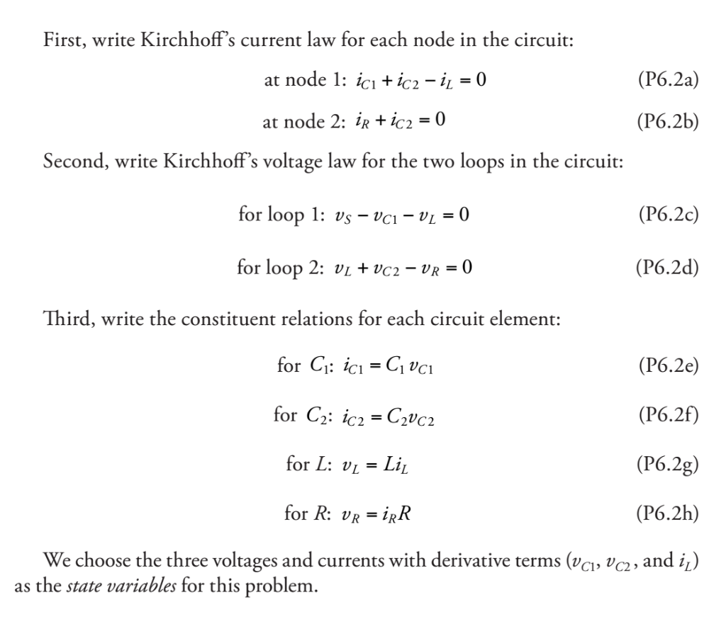
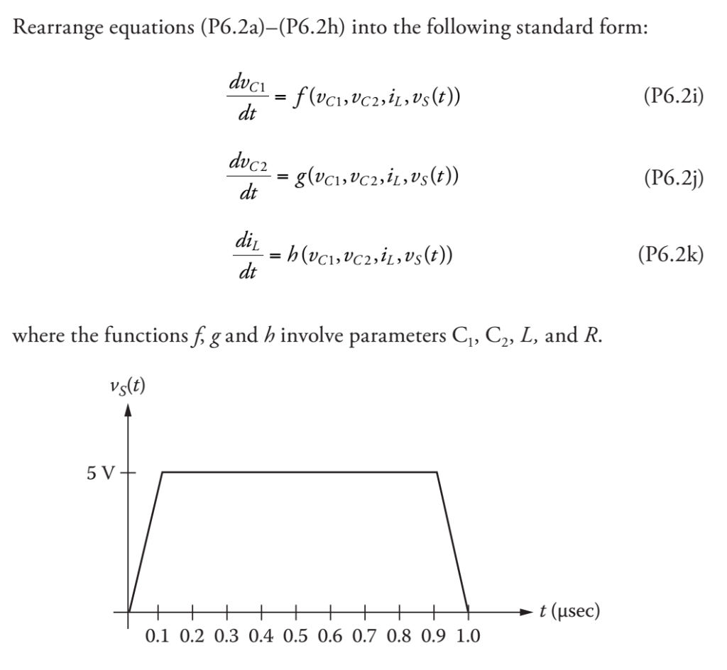
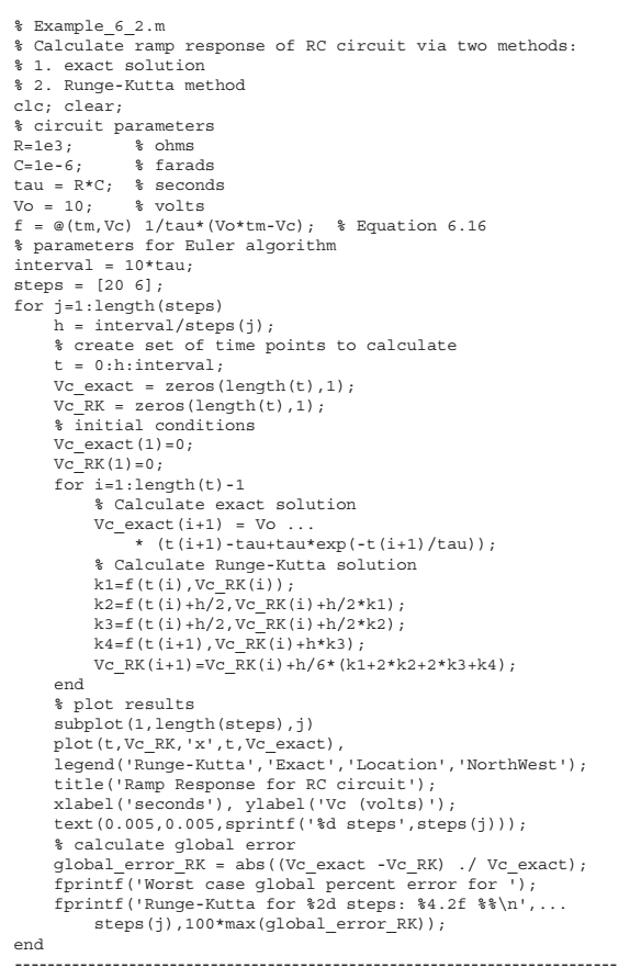
Project 6.2 Figure P6.2a shows a third-order RLC circuit. To run a time-domain transient anal- ysis, we transform the ci rcuit into differential equations using the following method: C1 C2 C1 C2 VL First, write Kirchhoff's current law for each node in the circuit: at node 1: ici +ic2 -iL - (P6.2a) at node 2: ie+ 2 = 0 (P6.2b) Second, write Kirchhoff's voltage law for the two loops in the circuit for loop 1: vs - vc1- vL-0 (P6.29 for loop 2: vi + vc2-UR 0 (P6.2d) Third, write the co nstituent relations for each circuit element (P6.2e) (P6.2f) (P6.2g) (P6.2h) We choose the three voltages and currents with derivative terms (vci vc2, and i,) for L: UL=LIL for R: UR=FR as the state variables for this problem Rearrange equations (P6.2a)-(P6.2h) into the following standard form dvc (P6.2i) = J (UCI, UC 2, IL, US(t)) dt dvc2 dt = g(UCI, UC 2 , IL, US(t)) (P6.2j) di (P6.2k) dt where the functionsfg and h involve parameters C1, C2, L, and R Vs(t) t (sec) 0.1 0.2 0.3 0.4 0.5 0.6 0.7 0.8 0.9 1.0 Solve Equations (P6.2i)-(P6.2k) with the Runge-Kutta algorithm for the fol- lowing circuit parameters: C1-1 F, C-0.001 F, R-100 kQ, L-0.01 se a time interval of 0 ts 10us and a step size of 0.01 us. Assume v(t is a 5-V pulse starting at time t 0 with rise time of 0.1 us, an "on" time of 0.8 us, and fall time of 0.1 us (as shown in Figure P6.2b). Initial conditions: vci(0)-0, vc2(0)-0, and i (0) 0 Plot on separate graphs: vci (t), VC2(t), L(t) and us (r) versus time %Example 6 2.m % Calculate ramp response of RC circuit via two methods % 1. exact solution % 2. Runge-Kutta method clc; clear; % circuit parameters R-1e3 C-1e-6 tau-R*C; % seconds Vo10 f-@(tm, Vc) 1/tau * (Vottm-Vc); % Equation 6.16 % parameters for Euler algorithm interval10*tau; steps[20 6] for j-l:length (steps) % ohms % farads % volts hinterval/steps (j) % create set of time points to calculate t0:h:interval; Vc_exact-zeros (length (t),1) Vc_RK zeros (length (t),1) % initial conditions Vc exact (1)-0 Vc RK (1) 0 for i=1: length (t)-1 % Calculate exact solution Vc_exact (i+1) Vo .. . *(t (i+1)-tau+tau*exp (-t (i+1) /tau)) % Calculate Runge-Kutta solution k1-f (t (i), Vc RK (i)) Vc_RK (i+1)-Vc_RK (i) +h/6 (k1+2 k2+2*k3+k4); end % plot results subplot (1,length (steps),j) plot (t,Vc RK, x't Vc exact) legend ('Runge-Kutta', 'Exact','Location', 'NorthWest') title ('Ramp Response for RC circuit') xlabel ('seconds, ylabel 'Vc (volts)') text (0. 005, 0 . 005, sprintf ( ' %d steps ' ' steps (j ) ) ) ; % calculate global error global error RK-abs ((Vc exact -Vc RK) ./Vvc exact) fprintf ('Worst case global percent error for '); fprintf ('Runge-Kutta for %2d steps: %4.2E %% ', steps (j),100 max (global_error_RK)); end Project 6.2 Figure P6.2a shows a third-order RLC circuit. To run a time-domain transient anal- ysis, we transform the ci rcuit into differential equations using the following method: C1 C2 C1 C2 VL First, write Kirchhoff's current law for each node in the circuit: at node 1: ici +ic2 -iL - (P6.2a) at node 2: ie+ 2 = 0 (P6.2b) Second, write Kirchhoff's voltage law for the two loops in the circuit for loop 1: vs - vc1- vL-0 (P6.29 for loop 2: vi + vc2-UR 0 (P6.2d) Third, write the co nstituent relations for each circuit element (P6.2e) (P6.2f) (P6.2g) (P6.2h) We choose the three voltages and currents with derivative terms (vci vc2, and i,) for L: UL=LIL for R: UR=FR as the state variables for this problem Rearrange equations (P6.2a)-(P6.2h) into the following standard form dvc (P6.2i) = J (UCI, UC 2, IL, US(t)) dt dvc2 dt = g(UCI, UC 2 , IL, US(t)) (P6.2j) di (P6.2k) dt where the functionsfg and h involve parameters C1, C2, L, and R Vs(t) t (sec) 0.1 0.2 0.3 0.4 0.5 0.6 0.7 0.8 0.9 1.0 Solve Equations (P6.2i)-(P6.2k) with the Runge-Kutta algorithm for the fol- lowing circuit parameters: C1-1 F, C-0.001 F, R-100 kQ, L-0.01 se a time interval of 0 ts 10us and a step size of 0.01 us. Assume v(t is a 5-V pulse starting at time t 0 with rise time of 0.1 us, an "on" time of 0.8 us, and fall time of 0.1 us (as shown in Figure P6.2b). Initial conditions: vci(0)-0, vc2(0)-0, and i (0) 0 Plot on separate graphs: vci (t), VC2(t), L(t) and us (r) versus time %Example 6 2.m % Calculate ramp response of RC circuit via two methods % 1. exact solution % 2. Runge-Kutta method clc; clear; % circuit parameters R-1e3 C-1e-6 tau-R*C; % seconds Vo10 f-@(tm, Vc) 1/tau * (Vottm-Vc); % Equation 6.16 % parameters for Euler algorithm interval10*tau; steps[20 6] for j-l:length (steps) % ohms % farads % volts hinterval/steps (j) % create set of time points to calculate t0:h:interval; Vc_exact-zeros (length (t),1) Vc_RK zeros (length (t),1) % initial conditions Vc exact (1)-0 Vc RK (1) 0 for i=1: length (t)-1 % Calculate exact solution Vc_exact (i+1) Vo .. . *(t (i+1)-tau+tau*exp (-t (i+1) /tau)) % Calculate Runge-Kutta solution k1-f (t (i), Vc RK (i)) Vc_RK (i+1)-Vc_RK (i) +h/6 (k1+2 k2+2*k3+k4); end % plot results subplot (1,length (steps),j) plot (t,Vc RK, x't Vc exact) legend ('Runge-Kutta', 'Exact','Location', 'NorthWest') title ('Ramp Response for RC circuit') xlabel ('seconds, ylabel 'Vc (volts)') text (0. 005, 0 . 005, sprintf ( ' %d steps ' ' steps (j ) ) ) ; % calculate global error global error RK-abs ((Vc exact -Vc RK) ./Vvc exact) fprintf ('Worst case global percent error for '); fprintf ('Runge-Kutta for %2d steps: %4.2E %% ', steps (j),100 max (global_error_RK)); end
