Please answer all. Tables posted if needed!
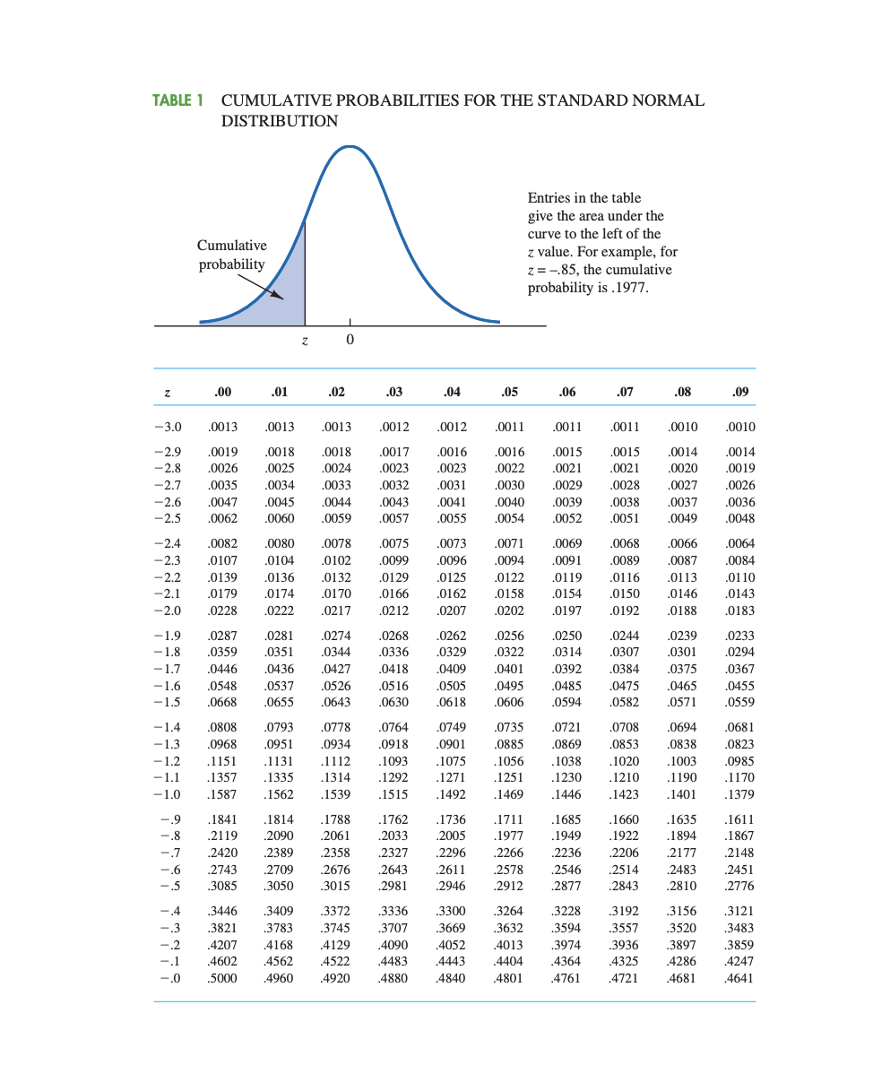
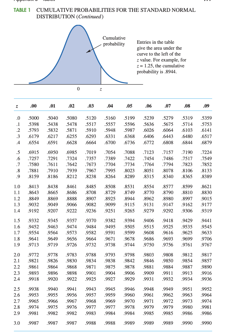
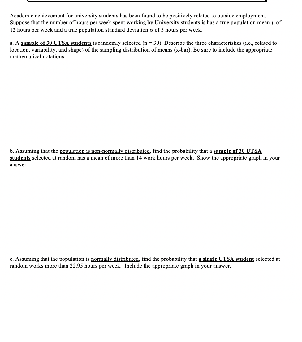
TABLE 1 CUMULATIVE PROBABILITIES FOR THE STANDARD NORMAL DISTRIBUTION Entries in the table give the area under the Cumulative curve to the left of the probability z value. For example, for z = -.85, the cumulative probability is . 1977. Z 0 .00 .01 .02 .03 .04 .05 06 .07 .08 .09 -3.0 .0013 .0013 .0013 .0011 001 1 .0011 0010 .0010 -2.9 0019 0018 .0017 0016 .0016 0015 0015 0014 0014 -2.8 0026 0025 0024 0023 0022 0021 0021 0020 0019 -2.7 .0035 1033 0032 0030 0029 0028 1027 0026 -2.6 0047 .0045 0044 0043 )040 0039 037 0036 -2.5 0062 0060 .0055 0054 0052 .0051 .0049 0048 -2.4 0082 .0080 0078 007 0071 0069 .0066 -2.3 .0107 .0104 .0102 .0099 0096 .0091 0089 .0087 0084 -2.2 0139 .0136 0132 0129 0125 0122 0119 0113 .0110 -2.1 0179 0174 0170 0162 0158 0154 .0150 .0146 0143 -2.0 0228 .0212 0207 .0197 .0188 0183 -1.9 .0287 0274 0262 .0256 0250 .0239 0233 -1.8 0359 .0351 0344 .0336 0329 0314 -1.7 .0446 0436 .0427 0409 040 0392 .0375 0367 -1.6 .0548 .0537 0526 0505 0495 0485 0475 .0465 0455 -1.5 .0668 0655 .0643 0630 0618 .0606 .0594 0582 .0571 0559 -1.4 0793 0778 0764 0735 .0721 0708 0681 -1.3 .0968 .0951 .0934 0901 0869 0853 0838 .0823 -1.2 .1151 1131 1112 1093 1075 1056 1038 1020 1003 0985 -1.1 .1292 1271 125 .1210 .1190 -1.0 1562 .1539 .1515 .1492 .1469 .1423 .1401 1379 -.9 .1814 .1762 .1736 1685 1660 .1635 .1611 -.8 .21 19 .2090 2005 1977 .1949 .1922 1894 1867 -.7 2420 .2358 2327 2296 .2266 2236 2206 2177 -.6 .2743 2709 2676 .2643 2546 .2514 .2483 .2451 - 5 .3085 3050 .3015 .2981 2946 .2912 2877 .2843 .2810 -.4 3409 3336 3300 .3264 3228 3192 .3121 .3821 .3745 3707 3669 .3632 3594 3557 .3520 3483 4207 4168 .4129 4052 4013 3974 .3936 4562 4522 4483 4443 4404 4364 4325 4286 4247 - 0 .5000 4960 .4920 .4880 .4840 .4801 4761 .4721 .4681 4641TABLE 1 CUMULATIVE PROBABILITIES FOR THE STANDARD NORMAL DISTRIBUTION (Continued) Entries in the table give the area under the curve to the left of the z value. For example, for z = 1.25, the cumulative probability is .8944. Z Z .00 .01 .02 .03 .04 .05 .06 .07 .08 .0 .5000 .5040 .5080 .5120 5160 .5319 .5359 .5438 5478 .5517 5557 .5596 5636 .5675 .5714 5793 .5832 5871 .5910 5948 6026 .6064 .6103 6141 6217 6255 .6293 6331 6368 .6406 .6443 .6480 .6517 4 6591 .6664 6736 .6772 .6808 .6844 .5 .6950 .6985 .7019 .7054 .7088 .7123 .7190 .6 .7291 .7324 7357 .7389 .7422 .7454 7517 .7549 .7580 .7611 .7642 .7673 .7704 .7734 .7764 .7794 .7823 .7852 .8 . 7881 .7910 7939 7967 .7995 8023 8051 .8078 .8106 .8133 .8159 .8186 8212 8264 .8340 .8365 8389 1.0 .8438 8461 8485 8508 8531 8554 .8577 .8599 .8621 1.1 .8665 8686 8708 8729 8749 8770 8790 .8810 .8830 1.2 .8849 8869 8888 8925 .8944 .8980 1.3 .9032 .9049 9066 9099 9131 .9147 .9162 .9177 1.4 .9192 .9207 .9222 .9236 .9251 .9265 .9279 .9292 .9306 9319 1.5 .9345 .9357 9370 .9382 9394 .9406 .9418 .9429 .9441 1.6 .9463 .9474 9484 .9495 9505 .9535 .9545 1.7 .9554 .9564 .9582 9591 9599 9608 .9616 .9625 .9633 1.8 9649 9656 .9671 .9678 .9686 .9693 .9699 9706 1.9 9719 9726 9732 9738 9744 9750 .9756 .9761 .9767 .9772 .9778 .9783 .9793 .9798 .9803 .9808 .9812 .9817 .9821 .9826 9830 9834 9838 9842 9846 .9850 .9854 9857 2.2 .9861 .9864 .9868 9871 9878 .9881 .9884 .9887 .9890 .9893 .9896 9898 9901 9904 9906 9909 9911 .9913 9916 2.4 .9920 9922 .9925 9927 .9929 .9934 .9936 2.5 .9938 9940 .9941 9943 .9945 .9946 .9948 .9949 .9951 .9952 2.6 .9953 9955 .9956 .9960 .9961 .9962 .9963 .9964 2.7 .9965 9966 9967 9968 9969 9971 .9972 .9973 9974 2.8 .9975 9978 .9980 9981 2.9 .9981 .9982 .9982 9983 9984 .9985 .9986 .9986 3.0 .9987 .9987 .9988 .9988 .9989 .9989 .9989 .9990 .9990Academic achievement for university students has been found to be positively related to outside employment. Suppose that the number of hours per week spent working by University students is has a true population mean u of 12 hours per week and a true population standard deviation 6 of 5 hours per week. a. A sample of 30 UTSA students is randomly selected (n = 30). Describe the three characteristics (i.e., related to location, variability, and shape) of the sampling distribution of means (x-bar). Be sure to include the appropriate mathematical notations. b. Assuming that the pgpulation is non-normally distributed, nd the probability that a sample of 30 UTSA students selected at random has a mean of more than 14 work hours per week. Show the appropriate graph in your answer. c. Assuming that the population is normally distributed, nd the probability that a single UTSA student selected at random works more than 22.95 hours per week. Include the appropriate graph in your