Please answer using R code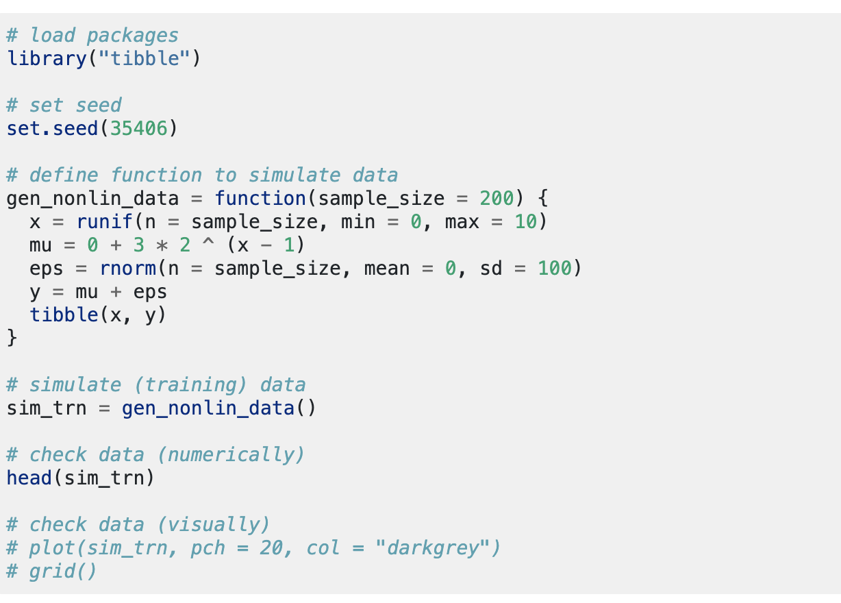
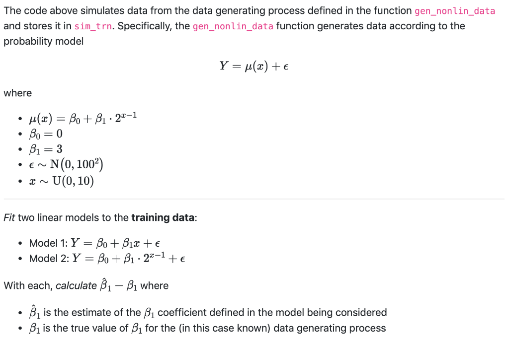
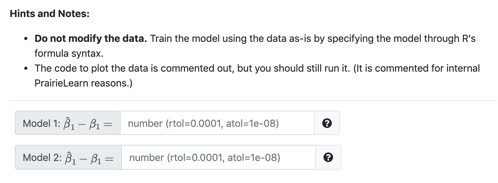
# load packages library("tibble") # set seed set.seed (35406) = #define function to simulate data gen_nonlin_data function(sample_size 200) { X = runifan sample_size, min = 0, max = 10) mu = 0 + 3 * 2 ^ (x - 1) eps = rnorm(n sample_size, mean = O, sd = 100) y = mu + eps tibble(x, y) } # simulate (training) data sim_trn gen_nonlin_data() = # check data (numerically) head (sim_trn) # check data (visually) # plot(sim_trn, pch = 20, col # grid() "darkgrey") The code above simulates data from the data generating process defined in the function gen_nonlin_data and stores it in sim_trn. Specifically, the gen_nonlin_data function generates data according to the probability model Y = u(x) + where . . u(x) = Be + B1. 221 Bo=0 Bi=3 N(0, 1002) U(0,10) EN Fit two linear models to the training data: Model 1: Y = Bo + B1x + Model 2: Y = Bo + B1. 221 + With each, calculate 1 - B1 where is the estimate of the B1 coefficient defined in the model being considered Bi is the true value of B1 for the (in this case known) data generating process Hints and Notes: Do not modify the data. Train the model using the data as-is by specifying the model through R's formula syntax. The code to plot the data is commented out, but you should still run it. (It is commented for internal PrairieLearn reasons.) Model 1: 1 B1 = number (rtol=0.0001, atol=1e-08) Model 2: B1 B1 = number (rtol=0.0001, atol=1e-08) # load packages library("tibble") # set seed set.seed (35406) = #define function to simulate data gen_nonlin_data function(sample_size 200) { X = runifan sample_size, min = 0, max = 10) mu = 0 + 3 * 2 ^ (x - 1) eps = rnorm(n sample_size, mean = O, sd = 100) y = mu + eps tibble(x, y) } # simulate (training) data sim_trn gen_nonlin_data() = # check data (numerically) head (sim_trn) # check data (visually) # plot(sim_trn, pch = 20, col # grid() "darkgrey") The code above simulates data from the data generating process defined in the function gen_nonlin_data and stores it in sim_trn. Specifically, the gen_nonlin_data function generates data according to the probability model Y = u(x) + where . . u(x) = Be + B1. 221 Bo=0 Bi=3 N(0, 1002) U(0,10) EN Fit two linear models to the training data: Model 1: Y = Bo + B1x + Model 2: Y = Bo + B1. 221 + With each, calculate 1 - B1 where is the estimate of the B1 coefficient defined in the model being considered Bi is the true value of B1 for the (in this case known) data generating process Hints and Notes: Do not modify the data. Train the model using the data as-is by specifying the model through R's formula syntax. The code to plot the data is commented out, but you should still run it. (It is commented for internal PrairieLearn reasons.) Model 1: 1 B1 = number (rtol=0.0001, atol=1e-08) Model 2: B1 B1 = number (rtol=0.0001, atol=1e-08)