Please answer within 10hrs and I'll give u thumbs up. First pic is the question and the other pic is previous question and answer for your reference. thank you.
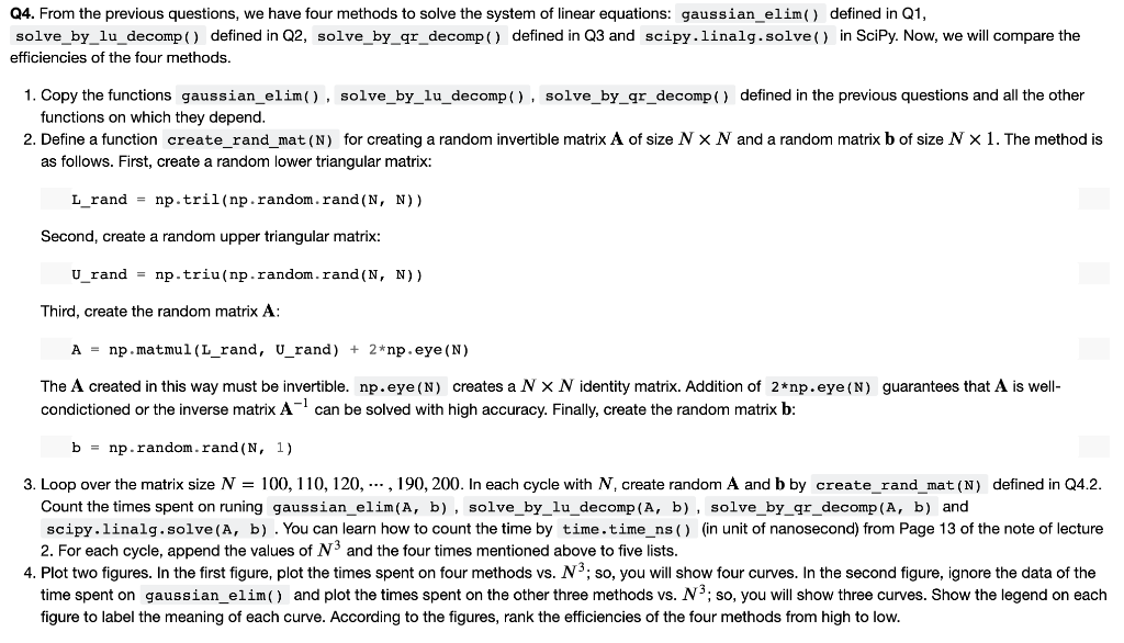
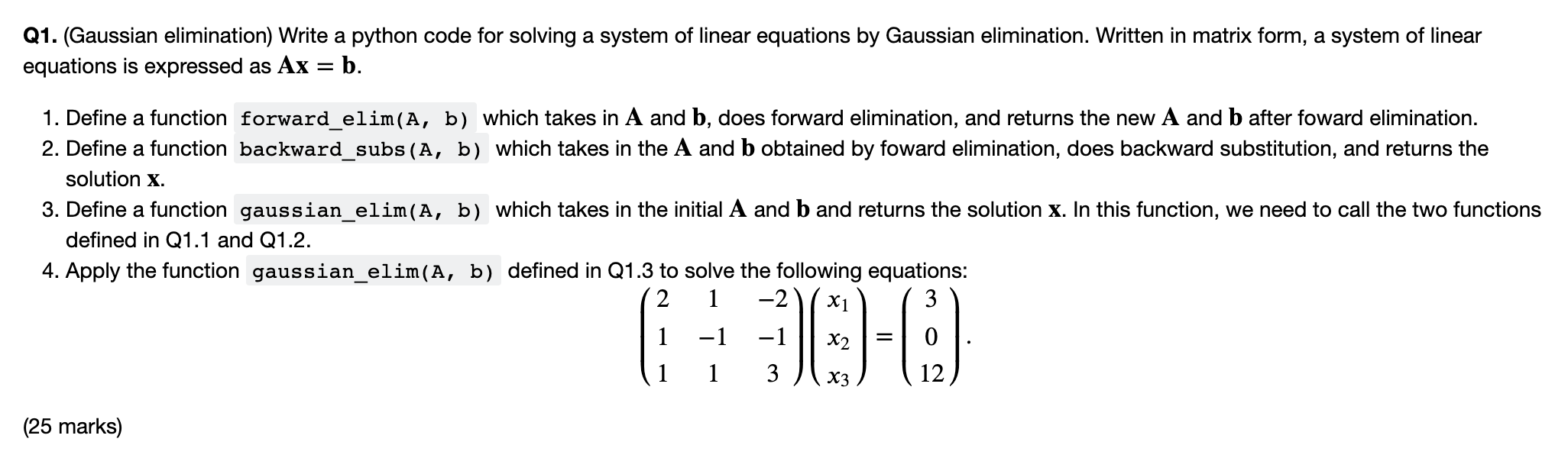
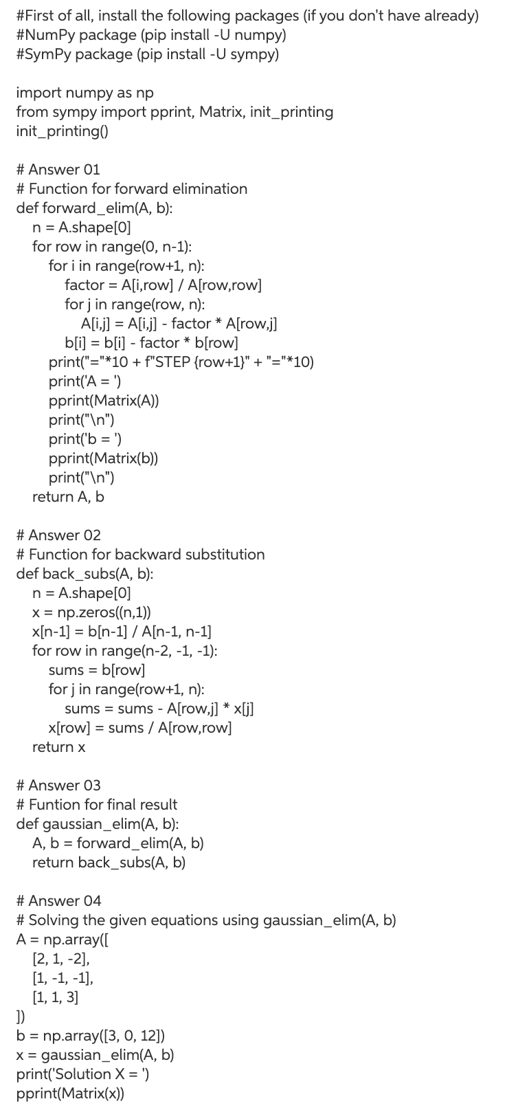
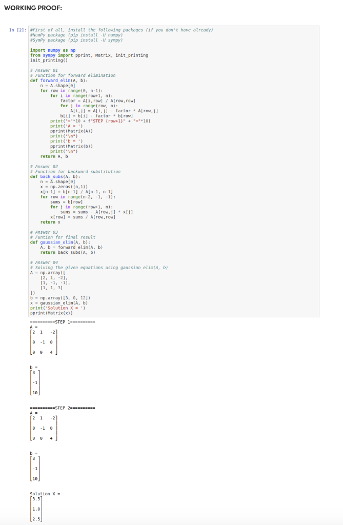
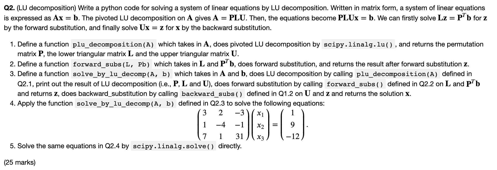
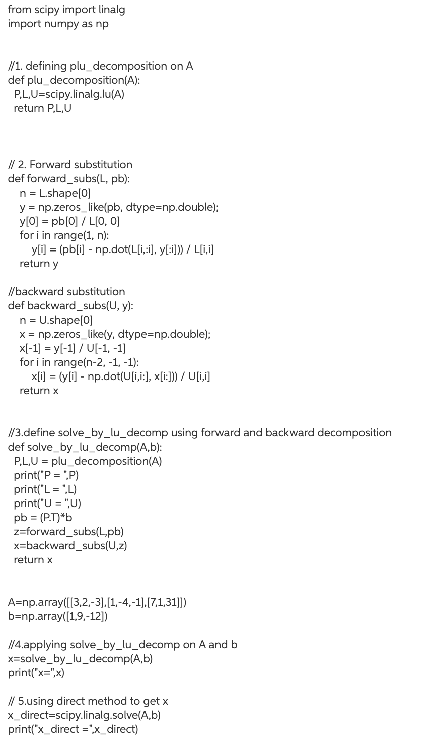
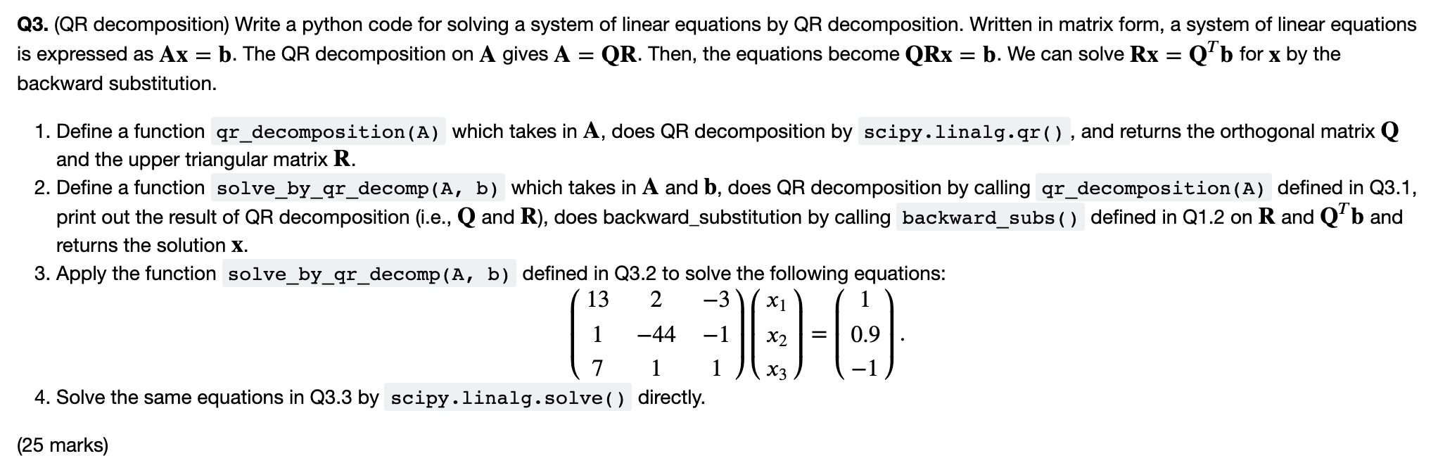
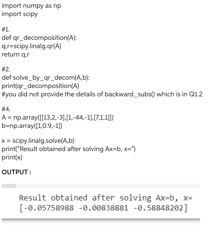
Q4. From the previous questions, we have four methods to solve the system of linear equations: gaussian_elim() defined in Q1, solve_by_lu_decomp() defined in Q2, solve_by_gr_decomp() defined in Q3 and scipy.linalg.solve()in SciPy. Now, we will compare the efficiencies of the four methods. 1. Copy the functions gaussian_elim() , solve_by_lu_decomp() , solve_by_gr_decomp() defined in the previous questions and all the other functions on which they depend. 2. Define a function create_rand_mat(n) for creating a random invertible matrix A of size NXN and a random matrix b of size N X 1. The method is as follows. First, create a random lower triangular matrix: L_rand = np.tril(np.random.rand (N, N)) Second, create a random upper triangular matrix: U_rand = np.triu(np.random.rand(N, N)) Third, create the random matrix A: A = np.matmul(L_rand, U_rand) + 2*np.eye (N) The A created in this way must be invertible. np.eye(N) creates a NX N identity matrix. Addition of 2*np.eye(N) guarantees that A is well- condictioned or the inverse matrix A can be solved with high accuracy. Finally, create the random matrix b: b = np.random.rand (N, 1) 3. Loop over the matrix size N = 100, 110, 120,.,190, 200. In each cycle with N, create random A and b by create_rand_mat(N) defined in Q4.2. Count the times spent on gaussian_elim(A, b), solve_by_lu_decomp (A, b), solve_by_gr_decomp (A, b) and scipy.linalg. solve(A, b). You can learn how to count the time by time.time_ns() (in unit of nanosecond) from Page 13 of the note of lecture 2. For each cycle, append the values of N3 and the four times mentioned above to five lists. 4. Plot two figures. In the first figure, plot the times spent on four methods vs. N; so, you will show four curves. In the second figure, ignore the data of the time spent on gaussian_elim() and plot the times spent on the other three methods vs. N3, so, you will show three curves. Show the legend on each figure to label the meaning of each curve. According to the figures, rank the efficiencies of the four methods from high to low. Q1. (Gaussian elimination) Write a python code for solving a system of linear equations by Gaussian elimination. Written in matrix form, a system of linear equations is expressed as Ax = b. 1. Define a function forward_elim(A, b) which takes in A and b, does forward elimination, and returns the new A and b after foward elimination. 2. Define a function backward_subs (A, b) which takes in the A and b obtained by foward elimination, does backward substitution, and returns the solution x. 3. Define a function gaussian_elim(A, b) which takes in the initial A and b and returns the solution x. In this function, we need to call the two functions defined in Q1.1 and Q1.2. 4. Apply the function gaussian_elim(A, b) defined in Q1.3 to solve the following equations: 2 1 -2 X1 3 1 -1 1 1 3 X3 12 (25 marks) First of all, install the following packages (if you don't have already) Numpy package (pip install -U numpy) Sympy package (pip install -U sympy) _mport numpy as np Erom sympy import pprint, Matrix, init_printing Enit_printing Answer 01 Function for forward elimination Hef forward_elim(a, b): n = A. shape[ 0 ] for row in range(0, n-1): for i in range (row+1, n): factor - Ali, row / A[row, row] for j in range (row, n): A[i,j] - A[i, j - factor A[row, j] b[i] = b[i] - factor + b[row] print("-"*10 + F"STEP {row+1}" + "-"*10) print('A=') pprint (Matrix(A)) print(" ") print('b =) pprint (Matrix(b)) print(" ") return A, b Answer 02 Function for backward substitution Bef back_subs (a, b): n = A. shape [0] x = np.zeros(in, 1)) x[n-1] = b[n-1] / A[n-1, n-1] for row in range (n-2, -1, -1): sums = b[row] for j in range (row+1, n): sums - sums - Afrow, j1 . xtil x[row) - sums / Acrow, row] return x Answer 03 Funtion for final result ief gaussian_elim(A,b): A, b = forward_elim(A, b) return back_subs(A, b) Answer 04 Solving the given equations using gaussian_elim(A, b) = np.array ( [2, 1, -2) [1,-1,-1], [1, 1, 31 1) = np.array([3,0, 121) - gaussian_elim(A, b) print('Solution x =) print (Matrix(x)) (()) WORKING PROOF: In [2]: #First of all, install the following packages (if you don't have already) #Numpy package (pip install -Ununpy) Symy package (pip install - sympy) import numpy as np from sympy import pprint, Matrix, init_printing init_printing) Answer 01 # Function for forward elimination det forward elin(a, b): n-A.shape[o] for row in range(0, n. 1): for i in range(rowl, n): factor = A[i, row / Afrow, row] for j in range(row, n): A[1.]] = A[1,1] - factor . A[row,j] b[1] = b[1] - factor - brow] print("*10 + f"STEP {row+1}" + ***10) print('A=') pprint (Matrix(A)) print(" ") print('b') pprint (Matrix(b)) print(" ") return Ab + Answer 62 # Function for backward substitution def back subs(A,b): n = A. shape[o] x = np.zeros(in, 1)) x[n 1] = b[n 1] / A(n-1, n-1] for row in range(n-2, 1, 1): sums = b[row] for j in range(row+1, n): suns = sums - Afrow.j] - x[i] x[row] = sums / A[row,row] return x # Answer 63 # Funtion for final result def gaussian_elin(a, b): A, b = forward elimi, b} return back_subs(A. b) Answer 04 Solving the given equations using gaussian elim/A, b) A = np.array ( [ [2, 1, -2). 11,-1,-1]. 11, 1, 31 b = np.array([3, 0, 121) X = gaussian elim(Ab) print('Solution X =) pprint (Matrix(x)) STEP 1- [21 -2 0-1 - 1 @ 4 10 ==========STEP 2 ========== A = 21 -2 D -1 0 Solution X - (3.51 1.0 2.5) Q2. (LU decomposition) Write a python code for solving a system of linear equations by LU decomposition. Written in matrix form, a system of linear equations is expressed as Ax = b. The pivoted LU decomposition on A gives A = PLU. Then, the equations become PLUX b. We can firstly solve Lz = PTb for z by the forward substitution, and finally solve Ux = z for x by the backward substitution. 1. Define a function plu_decomposition(A) which takes in A, does pivoted LU decomposition by scipy.linalg.lu(), and returns the permutation matrix P, the lower triangular matrix L and the upper triangular matrix U. 2. Define a function forward_subs(L, Pb) which takes in L and PTb, does forward substitution, and returns the result after forward substitution z. 3. Define a function solve_by_lu_decomp (A, b) which takes in A and b, does LU decomposition by calling plu_decomposition(A) defined in Q2.1, print out the result of LU decomposition (i.e., P, L and U), does forward substitution by calling forward_subs() defined in Q2.2 on L and Pb and returns z, does backward_substitution by calling backward_subs() defined in Q1.2 on U and z and returns the solution x. 4. Apply the function solve_by_lu_decomp (A, b) defined in Q2.3 to solve the following equations: 3 2 -3 X1 1 -4 -1 9 7 1 31 -12 5. Solve the same equations in Q2.4 by scipy.linalg.solve() directly. (25 marks) from scipy import linalg import numpy as np I/1. defining plu_decomposition on A def plu_decomposition(A): P,L,U=scipy.linalg.lu(A) return P,L,U // 2. Forward substitution def forward_subs(L, pb): n = L.shape[0] y = np.zeros_like(pb, dtype=np.double); y[0] = pb[0] / L[0, 0] for i in range(1, n): y[i] = (pb[i] - np.dot(L[i,:i], y[:i])) / L[i,i] return y //backward substitution def backward_subs(U, y): n = U.shape[0] x = np.zeros_likely, dtype=np.double); x[-1] = y(-1] / U[-1, -1] for i in range(n-2, -1, -1): x[i] = (y[i] - np.dot(U[i,i:], x[i:])) / U[i,i] return x //3.define solve_by_lu_decomp using forward and backward decomposition def solve_by_lu_decomp(A,b): P,L,U = plu_decomposition(A) print("P = "P) print("L = "L) print("U = "U) pb = (P.T)*b z=forward_subs(L,pb) x=backward_subs(U,z) return x A=np.array([[3,2,-3],[1,-4,-1],[7,1,31]]) b=np.array([1,9,-12]) 1/4.applying solve_by_lu_decomp on A and b x=solve_by_lu_decomp(A,b) print("x=",x) // 5.using direct method to get x x_direct=scipy.linalg.solve(A,b) print("x_direct =",x_direct) Q3. (QR decomposition) Write a python code for solving a system of linear equations by QR decomposition. Written in matrix form, a system of linear equations is expressed as Ax = b. The QR decomposition on A gives A = QR. Then, the equations become QRx = b. We can solve Rx = Qb for x by the backward substitution. 1. Define a function qr_decomposition(A) which takes in A, does QR decomposition by scipy.linalg.qr(), and returns the orthogonal matrix Q and the upper triangular matrix R. 2. Define a function solve_by_qr_decomp (A, b) which takes in A and b, does QR decomposition by calling gr_decomposition (A) defined in Q3.1, print out the result of QR decomposition (i.e., Q and R), does backward_substitution by calling backward_subs() defined in Q1.2 on R and Qb and returns the solution x. 3. Apply the function solve_by_qr_decomp (A, b) defined in Q3.2 to solve the following equations: 13 2 X1 1 -44 -1 X2 0.9 7 1 1 X3 4. Solve the same equations in Q3.3 by scipy.linalg.solve () directly. ( (25 marks) import numpy as np import scipy #1. def qr_decomposition(A): q,r=scipy.linalg.qr(A) return qr #2. def solve_by_qr_decom(A,b): print(qr_decomposition(A) #you did not provide the details of backward_subs() which is in Q1.2 #4. A = np.array([[13,2,-3],[1,-44,-1],[7,1,1]]) b=np.array([1,0.9,-1]) x = scipy.linalg.solve(A,b) print("Result obtained after solving Ax=b, x=") print(x) OUTPUT: Result obtained after solving Ax=b, x= [-0.05758988 -0.00838881 -0.58848202] Q4. From the previous questions, we have four methods to solve the system of linear equations: gaussian_elim() defined in Q1, solve_by_lu_decomp() defined in Q2, solve_by_gr_decomp() defined in Q3 and scipy.linalg.solve()in SciPy. Now, we will compare the efficiencies of the four methods. 1. Copy the functions gaussian_elim() , solve_by_lu_decomp() , solve_by_gr_decomp() defined in the previous questions and all the other functions on which they depend. 2. Define a function create_rand_mat(n) for creating a random invertible matrix A of size NXN and a random matrix b of size N X 1. The method is as follows. First, create a random lower triangular matrix: L_rand = np.tril(np.random.rand (N, N)) Second, create a random upper triangular matrix: U_rand = np.triu(np.random.rand(N, N)) Third, create the random matrix A: A = np.matmul(L_rand, U_rand) + 2*np.eye (N) The A created in this way must be invertible. np.eye(N) creates a NX N identity matrix. Addition of 2*np.eye(N) guarantees that A is well- condictioned or the inverse matrix A can be solved with high accuracy. Finally, create the random matrix b: b = np.random.rand (N, 1) 3. Loop over the matrix size N = 100, 110, 120,.,190, 200. In each cycle with N, create random A and b by create_rand_mat(N) defined in Q4.2. Count the times spent on gaussian_elim(A, b), solve_by_lu_decomp (A, b), solve_by_gr_decomp (A, b) and scipy.linalg. solve(A, b). You can learn how to count the time by time.time_ns() (in unit of nanosecond) from Page 13 of the note of lecture 2. For each cycle, append the values of N3 and the four times mentioned above to five lists. 4. Plot two figures. In the first figure, plot the times spent on four methods vs. N; so, you will show four curves. In the second figure, ignore the data of the time spent on gaussian_elim() and plot the times spent on the other three methods vs. N3, so, you will show three curves. Show the legend on each figure to label the meaning of each curve. According to the figures, rank the efficiencies of the four methods from high to low. Q1. (Gaussian elimination) Write a python code for solving a system of linear equations by Gaussian elimination. Written in matrix form, a system of linear equations is expressed as Ax = b. 1. Define a function forward_elim(A, b) which takes in A and b, does forward elimination, and returns the new A and b after foward elimination. 2. Define a function backward_subs (A, b) which takes in the A and b obtained by foward elimination, does backward substitution, and returns the solution x. 3. Define a function gaussian_elim(A, b) which takes in the initial A and b and returns the solution x. In this function, we need to call the two functions defined in Q1.1 and Q1.2. 4. Apply the function gaussian_elim(A, b) defined in Q1.3 to solve the following equations: 2 1 -2 X1 3 1 -1 1 1 3 X3 12 (25 marks) First of all, install the following packages (if you don't have already) Numpy package (pip install -U numpy) Sympy package (pip install -U sympy) _mport numpy as np Erom sympy import pprint, Matrix, init_printing Enit_printing Answer 01 Function for forward elimination Hef forward_elim(a, b): n = A. shape[ 0 ] for row in range(0, n-1): for i in range (row+1, n): factor - Ali, row / A[row, row] for j in range (row, n): A[i,j] - A[i, j - factor A[row, j] b[i] = b[i] - factor + b[row] print("-"*10 + F"STEP {row+1}" + "-"*10) print('A=') pprint (Matrix(A)) print(" ") print('b =) pprint (Matrix(b)) print(" ") return A, b Answer 02 Function for backward substitution Bef back_subs (a, b): n = A. shape [0] x = np.zeros(in, 1)) x[n-1] = b[n-1] / A[n-1, n-1] for row in range (n-2, -1, -1): sums = b[row] for j in range (row+1, n): sums - sums - Afrow, j1 . xtil x[row) - sums / Acrow, row] return x Answer 03 Funtion for final result ief gaussian_elim(A,b): A, b = forward_elim(A, b) return back_subs(A, b) Answer 04 Solving the given equations using gaussian_elim(A, b) = np.array ( [2, 1, -2) [1,-1,-1], [1, 1, 31 1) = np.array([3,0, 121) - gaussian_elim(A, b) print('Solution x =) print (Matrix(x)) (()) WORKING PROOF: In [2]: #First of all, install the following packages (if you don't have already) #Numpy package (pip install -Ununpy) Symy package (pip install - sympy) import numpy as np from sympy import pprint, Matrix, init_printing init_printing) Answer 01 # Function for forward elimination det forward elin(a, b): n-A.shape[o] for row in range(0, n. 1): for i in range(rowl, n): factor = A[i, row / Afrow, row] for j in range(row, n): A[1.]] = A[1,1] - factor . A[row,j] b[1] = b[1] - factor - brow] print("*10 + f"STEP {row+1}" + ***10) print('A=') pprint (Matrix(A)) print(" ") print('b') pprint (Matrix(b)) print(" ") return Ab + Answer 62 # Function for backward substitution def back subs(A,b): n = A. shape[o] x = np.zeros(in, 1)) x[n 1] = b[n 1] / A(n-1, n-1] for row in range(n-2, 1, 1): sums = b[row] for j in range(row+1, n): suns = sums - Afrow.j] - x[i] x[row] = sums / A[row,row] return x # Answer 63 # Funtion for final result def gaussian_elin(a, b): A, b = forward elimi, b} return back_subs(A. b) Answer 04 Solving the given equations using gaussian elim/A, b) A = np.array ( [ [2, 1, -2). 11,-1,-1]. 11, 1, 31 b = np.array([3, 0, 121) X = gaussian elim(Ab) print('Solution X =) pprint (Matrix(x)) STEP 1- [21 -2 0-1 - 1 @ 4 10 ==========STEP 2 ========== A = 21 -2 D -1 0 Solution X - (3.51 1.0 2.5) Q2. (LU decomposition) Write a python code for solving a system of linear equations by LU decomposition. Written in matrix form, a system of linear equations is expressed as Ax = b. The pivoted LU decomposition on A gives A = PLU. Then, the equations become PLUX b. We can firstly solve Lz = PTb for z by the forward substitution, and finally solve Ux = z for x by the backward substitution. 1. Define a function plu_decomposition(A) which takes in A, does pivoted LU decomposition by scipy.linalg.lu(), and returns the permutation matrix P, the lower triangular matrix L and the upper triangular matrix U. 2. Define a function forward_subs(L, Pb) which takes in L and PTb, does forward substitution, and returns the result after forward substitution z. 3. Define a function solve_by_lu_decomp (A, b) which takes in A and b, does LU decomposition by calling plu_decomposition(A) defined in Q2.1, print out the result of LU decomposition (i.e., P, L and U), does forward substitution by calling forward_subs() defined in Q2.2 on L and Pb and returns z, does backward_substitution by calling backward_subs() defined in Q1.2 on U and z and returns the solution x. 4. Apply the function solve_by_lu_decomp (A, b) defined in Q2.3 to solve the following equations: 3 2 -3 X1 1 -4 -1 9 7 1 31 -12 5. Solve the same equations in Q2.4 by scipy.linalg.solve() directly. (25 marks) from scipy import linalg import numpy as np I/1. defining plu_decomposition on A def plu_decomposition(A): P,L,U=scipy.linalg.lu(A) return P,L,U // 2. Forward substitution def forward_subs(L, pb): n = L.shape[0] y = np.zeros_like(pb, dtype=np.double); y[0] = pb[0] / L[0, 0] for i in range(1, n): y[i] = (pb[i] - np.dot(L[i,:i], y[:i])) / L[i,i] return y //backward substitution def backward_subs(U, y): n = U.shape[0] x = np.zeros_likely, dtype=np.double); x[-1] = y(-1] / U[-1, -1] for i in range(n-2, -1, -1): x[i] = (y[i] - np.dot(U[i,i:], x[i:])) / U[i,i] return x //3.define solve_by_lu_decomp using forward and backward decomposition def solve_by_lu_decomp(A,b): P,L,U = plu_decomposition(A) print("P = "P) print("L = "L) print("U = "U) pb = (P.T)*b z=forward_subs(L,pb) x=backward_subs(U,z) return x A=np.array([[3,2,-3],[1,-4,-1],[7,1,31]]) b=np.array([1,9,-12]) 1/4.applying solve_by_lu_decomp on A and b x=solve_by_lu_decomp(A,b) print("x=",x) // 5.using direct method to get x x_direct=scipy.linalg.solve(A,b) print("x_direct =",x_direct) Q3. (QR decomposition) Write a python code for solving a system of linear equations by QR decomposition. Written in matrix form, a system of linear equations is expressed as Ax = b. The QR decomposition on A gives A = QR. Then, the equations become QRx = b. We can solve Rx = Qb for x by the backward substitution. 1. Define a function qr_decomposition(A) which takes in A, does QR decomposition by scipy.linalg.qr(), and returns the orthogonal matrix Q and the upper triangular matrix R. 2. Define a function solve_by_qr_decomp (A, b) which takes in A and b, does QR decomposition by calling gr_decomposition (A) defined in Q3.1, print out the result of QR decomposition (i.e., Q and R), does backward_substitution by calling backward_subs() defined in Q1.2 on R and Qb and returns the solution x. 3. Apply the function solve_by_qr_decomp (A, b) defined in Q3.2 to solve the following equations: 13 2 X1 1 -44 -1 X2 0.9 7 1 1 X3 4. Solve the same equations in Q3.3 by scipy.linalg.solve () directly. ( (25 marks) import numpy as np import scipy #1. def qr_decomposition(A): q,r=scipy.linalg.qr(A) return qr #2. def solve_by_qr_decom(A,b): print(qr_decomposition(A) #you did not provide the details of backward_subs() which is in Q1.2 #4. A = np.array([[13,2,-3],[1,-44,-1],[7,1,1]]) b=np.array([1,0.9,-1]) x = scipy.linalg.solve(A,b) print("Result obtained after solving Ax=b, x=") print(x) OUTPUT: Result obtained after solving Ax=b, x= [-0.05758988 -0.00838881 -0.58848202]