Please calculate the WACC for the cash flows originating in Brazil, Argentina and Chile from a local perspective and from a US $ perspective. The data is below
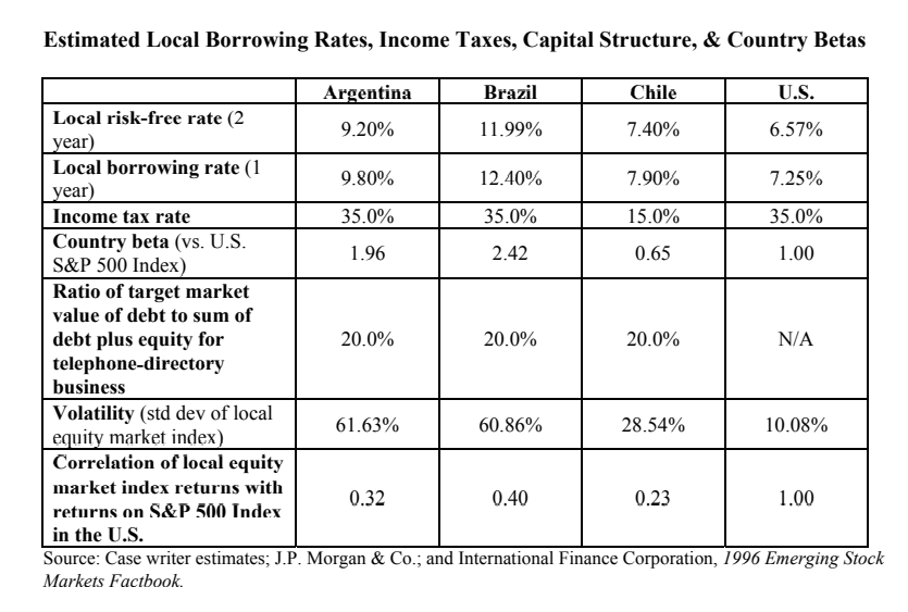
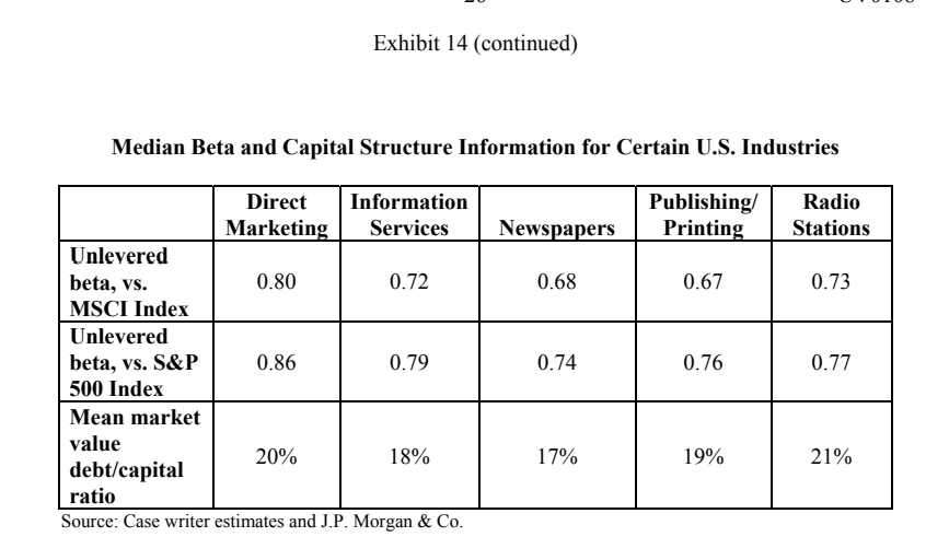
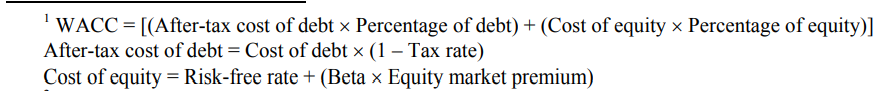
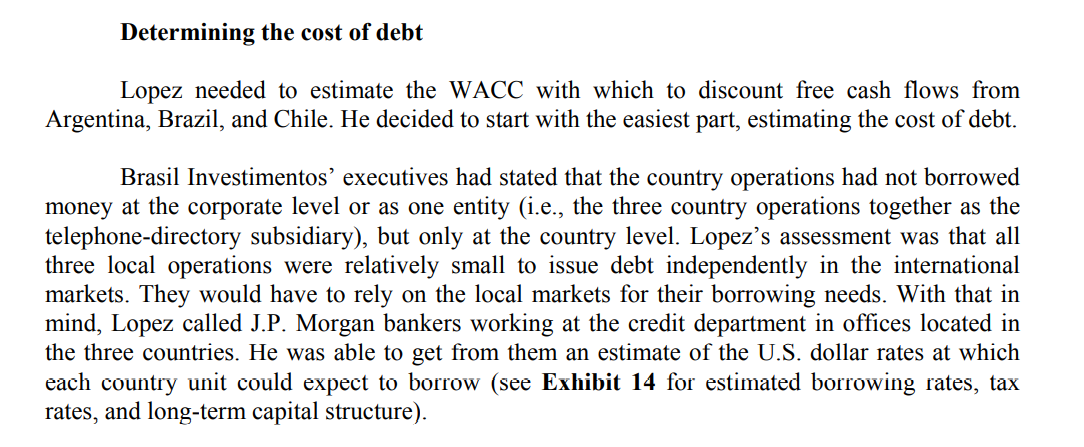
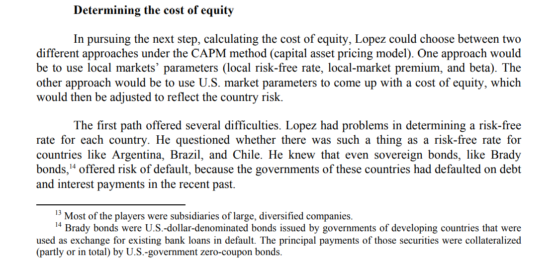
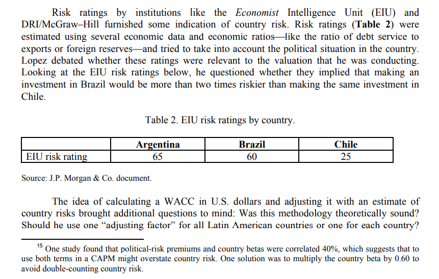
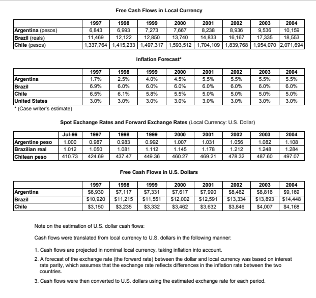
Estimated Local Borrowing Rates, Income Taxes, Capital Structure, & Country Betas Argentina Brazil Chile U.S. Local risk-free rate (2 9.20% 11.99% 7.40% 6.57% year) Local borrowing rate (1 9.80% 12.40% 7.90% 7.25% year) Income tax rate 35.0% 35.0% 15.0% 35.0% Country beta (vs. U.S. 1.96 2.42 0.65 1.00 S&P 500 Index) Ratio of target market value of debt to sum of debt plus equity for 20.0% 20.0% 20.0% N/A telephone-directory business Volatility (std dev of local 61.63% 60.86% 28.54% 10.08% equity market index) Correlation of local equity market index returns with 0.32 0.40 0.23 1.00 returns on S&P 500 Index in the U.S. Source: Case writer estimates; J.P. Morgan & Co.; and International Finance Corporation, 1996 Emerging Stock Markets Factbook. Exhibit 14 (continued) Median Beta and Capital Structure Information for Certain U.S. Industries Publishing Printing Radio Stations Newspapers 0.68 0.67 0.73 Direct Information Marketing Services Unlevered beta, vs. 0.80 0.72 MSCI Index Unlevered beta, vs. S&P 0.86 0.79 500 Index Mean market value 20% 18% debt/capital ratio Source: Case writer estimates and J.P. Morgan & Co. 0.74 0.76 0.77 17% 19% 21% WACC = [(After-tax cost of debt > Percentage of debt) + (Cost of equity ~ Percentage of equity)] After-tax cost of debt = Cost of debt x (1 Tax rate) Cost of equity = Risk-free rate + (Beta x Equity market premium) Determining the cost of debt Lopez needed to estimate the WACC with which to discount free cash flows from Argentina, Brazil, and Chile. He decided to start with the easiest part, estimating the cost of debt. Brasil Investimentos' executives had stated that the country operations had not borrowed money at the corporate level or as one entity (i.e., the three country operations together as the telephone-directory subsidiary), but only at the country level. Lopez's assessment was that all three local operations were relatively small to issue debt independently in the international markets. They would have to rely on the local markets for their borrowing needs. With that in mind, Lopez called J.P. Morgan bankers working at the credit department in offices located in the three countries. He was able to get from them an estimate of the U.S. dollar rates at which each country unit could expect to borrow (see Exhibit 14 for estimated borrowing rates, tax rates, and long-term capital structure). Determining the cost of equity In pursuing the next step, calculating the cost of equity, Lopez could choose between two different approaches under the CAPM method (capital asset pricing model). One approach would be to use local markets' parameters (local risk-free rate, local-market premium, and beta). The other approach would be to use U.S. market parameters to come up with a cost of equity, which would then be adjusted to reflect the country risk. The first path offered several difficulties. Lopez had problems in determining a risk-free rate for each country. He questioned whether there was such a thing as a risk-free rate for countries like Argentina, Brazil, and Chile. He knew that even sovereign bonds, like Brady bonds, 14 offered risk of default, because the governments of these countries had defaulted on debt and interest payments in the recent past. 13 14 Most of the players were subsidiaries of large, diversified companies. Brady bonds were U.S.-dollar-denominated bonds issued by governments of developing countries that were used as exchange for existing bank loans in default. The principal payments of those securities were collateralized (partly or in total) by U.S.-government zero-coupon bonds. Risk ratings by institutions like the Economist Intelligence Unit (EIU) and DRI/McGraw-Hill furnished some indication of country risk. Risk ratings (Table 2) were estimated using several economic data and economic ratios-like the ratio of debt service to exports or foreign reservesand tried to take into account the political situation in the country. Lopez debated whether these ratings were relevant to the valuation that he was conducting. Looking at the EI risk ratings below, he questioned whether they implied that making an investment in Brazil would be more than two times riskier than making the same investment in Chile. Table 2. EIU risk ratings by country. Argentina 65 Brazil 60 Chile 25 EIU risk rating Source: J.P. Morgan & Co. document. The idea of calculating a WACC in U.S. dollars and adjusting it with an estimate of country risks brought additional questions to mind: Was this methodology theoretically sound? Should he use one "adjusting factor for all Latin American countries or one for each country? 15 One study found that political-risk premiums and country betas were correlated 40%, which suggests that to use both terms in a CAPM might overstate country risk. One solution was to multiply the country beta by 0.60 to avoid double-counting country risk. Should the estimate of country risk used be the same, regardless of whether the investor is foreign or local? Should the discount rate be estimated using U.S.-market parameters even when one is dealing with a local prospective buyer? Conclusion Lopez returned to consider the DCF values in Exhibits 2, 3, and 4. Given an estimate of the investors' required rates of return on investments in Argentina, Brazil, and Chile, he could determine the value of each segment in U.S. dollars. The key issue, then, was to find the appropriate required rate of return for the telephone-directory business in each country. Free Cash Flows in Local Currency Argentina (pesos) Brazil (reals) Chile (pesos) 1997 1998 1999 2000 2001 2002 2003 2004 6,843 6,993 7.273 7.667 8.238 8.936 9,536 10,159 11,469 12,122 12.850 13,740 14,833 16,167 17,335 18,553 1,337,764 1,415,233 1,497,317 1,593,5121,704,109 1,839,768 1,954,070 2,071,694 Inflation Forecast Argentina Brazil Chile United States * (Case writer's estimate) 1997 1.7% 6.9% 6.5% 3.0% 1998 2.5% 6.0% 6.1% 3.0% 1999 4.0% 6.0% 5.8% 3.0% 2000 4.5% 6.0% 5.5% 3.0% 2001 5.5% 6.0% 5.0% 3.0% 2002 5.5% 6.0% 5.0% 3.0% 2003 5.5% 6.0% 5.0% 3.0% 2004 5.5% 6.0% 5.0% 3.0% Spot Exchange Rates and Forward Exchange Rates (Local Currency: U.S. Dollar) Argentine peso Brazilian real Chilean peso Jul-96 1.000 1.012 410.73 1997 0.987 1.050 424.69 1998 0.983 1.081 437.47 1999 0.992 1.112 449.36 2000 1.007 1.145 460 27 2001 1.031 1.178 469.21 2002 1.056 1.212 478.32 2003 1.082 1.248 487.60 2004 1.108 1.284 497.07 Free Cash Flows in U.S. Dollars Argentina Brazil Chile 1997 $6,930 $10.920 $3,150 1998 $7,117 $11,215 $3,235 1999 $7,331 $11,551 $3,332 2000 $7,617 $12,002 $3,462 2001 $7,990 $12,591 $3,632 2002 $8,462 $13,334 $3,846 2003 $8,816 $13,893 $4,007 2004 $9,169 $14,448 $4,168 Note on the estimation of U.S. dollar cash flows: Cash flows were translated from local currency to U.S. dollars in the following manner: 1. Cash flows are projected in nominal local currency, taking inflation into account. 2. A forecast of the exchange rate the forward rate) between the dollar and local currency was based on interest rate parity, which assumes that the exchange rate reflects differences in the inflation rate between the two countries. 3. Cash flows were then converted to U.S. dollars using the estimated exchange rate for each period. Estimated Local Borrowing Rates, Income Taxes, Capital Structure, & Country Betas Argentina Brazil Chile U.S. Local risk-free rate (2 9.20% 11.99% 7.40% 6.57% year) Local borrowing rate (1 9.80% 12.40% 7.90% 7.25% year) Income tax rate 35.0% 35.0% 15.0% 35.0% Country beta (vs. U.S. 1.96 2.42 0.65 1.00 S&P 500 Index) Ratio of target market value of debt to sum of debt plus equity for 20.0% 20.0% 20.0% N/A telephone-directory business Volatility (std dev of local 61.63% 60.86% 28.54% 10.08% equity market index) Correlation of local equity market index returns with 0.32 0.40 0.23 1.00 returns on S&P 500 Index in the U.S. Source: Case writer estimates; J.P. Morgan & Co.; and International Finance Corporation, 1996 Emerging Stock Markets Factbook. Exhibit 14 (continued) Median Beta and Capital Structure Information for Certain U.S. Industries Publishing Printing Radio Stations Newspapers 0.68 0.67 0.73 Direct Information Marketing Services Unlevered beta, vs. 0.80 0.72 MSCI Index Unlevered beta, vs. S&P 0.86 0.79 500 Index Mean market value 20% 18% debt/capital ratio Source: Case writer estimates and J.P. Morgan & Co. 0.74 0.76 0.77 17% 19% 21% WACC = [(After-tax cost of debt > Percentage of debt) + (Cost of equity ~ Percentage of equity)] After-tax cost of debt = Cost of debt x (1 Tax rate) Cost of equity = Risk-free rate + (Beta x Equity market premium) Determining the cost of debt Lopez needed to estimate the WACC with which to discount free cash flows from Argentina, Brazil, and Chile. He decided to start with the easiest part, estimating the cost of debt. Brasil Investimentos' executives had stated that the country operations had not borrowed money at the corporate level or as one entity (i.e., the three country operations together as the telephone-directory subsidiary), but only at the country level. Lopez's assessment was that all three local operations were relatively small to issue debt independently in the international markets. They would have to rely on the local markets for their borrowing needs. With that in mind, Lopez called J.P. Morgan bankers working at the credit department in offices located in the three countries. He was able to get from them an estimate of the U.S. dollar rates at which each country unit could expect to borrow (see Exhibit 14 for estimated borrowing rates, tax rates, and long-term capital structure). Determining the cost of equity In pursuing the next step, calculating the cost of equity, Lopez could choose between two different approaches under the CAPM method (capital asset pricing model). One approach would be to use local markets' parameters (local risk-free rate, local-market premium, and beta). The other approach would be to use U.S. market parameters to come up with a cost of equity, which would then be adjusted to reflect the country risk. The first path offered several difficulties. Lopez had problems in determining a risk-free rate for each country. He questioned whether there was such a thing as a risk-free rate for countries like Argentina, Brazil, and Chile. He knew that even sovereign bonds, like Brady bonds, 14 offered risk of default, because the governments of these countries had defaulted on debt and interest payments in the recent past. 13 14 Most of the players were subsidiaries of large, diversified companies. Brady bonds were U.S.-dollar-denominated bonds issued by governments of developing countries that were used as exchange for existing bank loans in default. The principal payments of those securities were collateralized (partly or in total) by U.S.-government zero-coupon bonds. Risk ratings by institutions like the Economist Intelligence Unit (EIU) and DRI/McGraw-Hill furnished some indication of country risk. Risk ratings (Table 2) were estimated using several economic data and economic ratios-like the ratio of debt service to exports or foreign reservesand tried to take into account the political situation in the country. Lopez debated whether these ratings were relevant to the valuation that he was conducting. Looking at the EI risk ratings below, he questioned whether they implied that making an investment in Brazil would be more than two times riskier than making the same investment in Chile. Table 2. EIU risk ratings by country. Argentina 65 Brazil 60 Chile 25 EIU risk rating Source: J.P. Morgan & Co. document. The idea of calculating a WACC in U.S. dollars and adjusting it with an estimate of country risks brought additional questions to mind: Was this methodology theoretically sound? Should he use one "adjusting factor for all Latin American countries or one for each country? 15 One study found that political-risk premiums and country betas were correlated 40%, which suggests that to use both terms in a CAPM might overstate country risk. One solution was to multiply the country beta by 0.60 to avoid double-counting country risk. Should the estimate of country risk used be the same, regardless of whether the investor is foreign or local? Should the discount rate be estimated using U.S.-market parameters even when one is dealing with a local prospective buyer? Conclusion Lopez returned to consider the DCF values in Exhibits 2, 3, and 4. Given an estimate of the investors' required rates of return on investments in Argentina, Brazil, and Chile, he could determine the value of each segment in U.S. dollars. The key issue, then, was to find the appropriate required rate of return for the telephone-directory business in each country. Free Cash Flows in Local Currency Argentina (pesos) Brazil (reals) Chile (pesos) 1997 1998 1999 2000 2001 2002 2003 2004 6,843 6,993 7.273 7.667 8.238 8.936 9,536 10,159 11,469 12,122 12.850 13,740 14,833 16,167 17,335 18,553 1,337,764 1,415,233 1,497,317 1,593,5121,704,109 1,839,768 1,954,070 2,071,694 Inflation Forecast Argentina Brazil Chile United States * (Case writer's estimate) 1997 1.7% 6.9% 6.5% 3.0% 1998 2.5% 6.0% 6.1% 3.0% 1999 4.0% 6.0% 5.8% 3.0% 2000 4.5% 6.0% 5.5% 3.0% 2001 5.5% 6.0% 5.0% 3.0% 2002 5.5% 6.0% 5.0% 3.0% 2003 5.5% 6.0% 5.0% 3.0% 2004 5.5% 6.0% 5.0% 3.0% Spot Exchange Rates and Forward Exchange Rates (Local Currency: U.S. Dollar) Argentine peso Brazilian real Chilean peso Jul-96 1.000 1.012 410.73 1997 0.987 1.050 424.69 1998 0.983 1.081 437.47 1999 0.992 1.112 449.36 2000 1.007 1.145 460 27 2001 1.031 1.178 469.21 2002 1.056 1.212 478.32 2003 1.082 1.248 487.60 2004 1.108 1.284 497.07 Free Cash Flows in U.S. Dollars Argentina Brazil Chile 1997 $6,930 $10.920 $3,150 1998 $7,117 $11,215 $3,235 1999 $7,331 $11,551 $3,332 2000 $7,617 $12,002 $3,462 2001 $7,990 $12,591 $3,632 2002 $8,462 $13,334 $3,846 2003 $8,816 $13,893 $4,007 2004 $9,169 $14,448 $4,168 Note on the estimation of U.S. dollar cash flows: Cash flows were translated from local currency to U.S. dollars in the following manner: 1. Cash flows are projected in nominal local currency, taking inflation into account. 2. A forecast of the exchange rate the forward rate) between the dollar and local currency was based on interest rate parity, which assumes that the exchange rate reflects differences in the inflation rate between the two countries. 3. Cash flows were then converted to U.S. dollars using the estimated exchange rate for each period