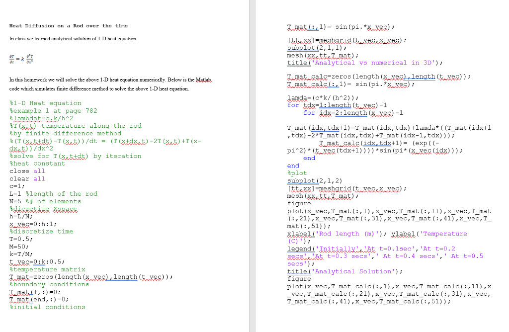
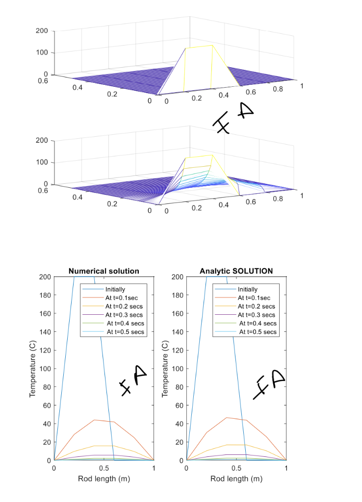
Please change the following code to help me obtain the graphs posted below

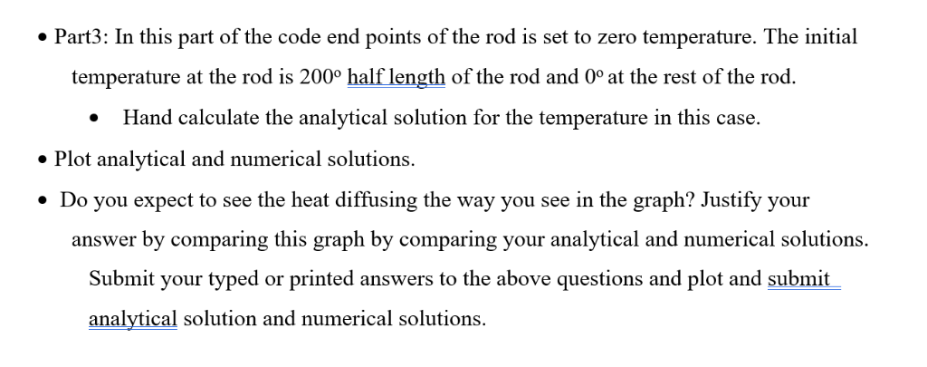
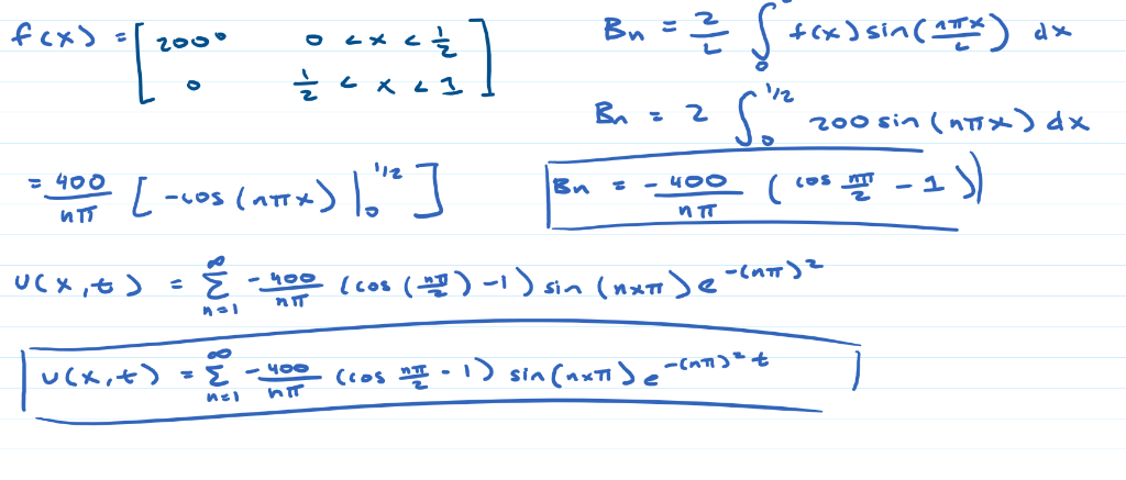
Heat Diffusion on a Rod over the time In class we learned analytical solution of 1-D heat equation subplot (2,1,1); aa7 le ('Analytical vs numerical in 3D In this homework we will solve the above 1-D heat equation numerically. Below is the Matlab code which simulates finite difference method to solve the above 1-D heat equation T mat salc-zeros (length ( veL length tveg)) Tmat sals(,1)- sin(pi.*x vec)i Lauda= (c*k/ (h^2) ) ; for tdx=1: length (tvec)-1 1-D Heat equation example 1 at page 782 lambdat-c.k/h 2 T) temperature along the rod %by finite difference method for id-2:length (ve)-1 T mat (idx, tdx+1)-T mat (idx, tdx) +lamda* ((T mat (idx+1 , tdx)-2*T mat (idx, tdx) +T mat (idx-1,tdx)) (idx, tdx+1)(exp (( p"2)" (Lyes (tax+1 ) ) ) ) *Sin (pi* (a.xes (dd8) ) ) ; solve for T (auktd5) by iteration end heat constant close all clear all c=1; L-1 %length of the rod N=5 of elements end plot subplot (2,1,2) figure plot (x_vec, T_mat (:,1),x_vec,T_mat (:,11),x_vec, T_mat (:,21),x_vec, T_mat (:,31), x_vec,T mat (:,41),x_vec, T mat (, 51)); xlabel ('Rod length (m)' ylabel ('Temperature h-L/N; discretize T-0.5 M=50; k-T/Mi time legend(' InitiallAt t-0.1sec,'At t-0.2 secs'. At t-0.3 secs'.' At t-0.4 secs'.' At t-0.5 secs title ('Analytical Solution') figure plot (x vec,T mat calc(:.1)x vec.T mat calc(.11).x vec,Tmat_calc(:,21),xvec, T mat_calc (:,31), x_vec, T_mat_calc(,41),x_vec,T_mat_calc(:,51)); temperature matrix mat-zeros (length (zveg) lenqth (tves)) boundary conditions Tmat (end,)0 initial conditions xlabel(' Rod length (m) '); ylabel ('Temperature legend (' Tnitiallyit t-0.1sec", 'At t-0.2 SeGsAt t-0.3 secs', At t-0.4 secs,At t 0.5 secs) title('Numerical Solution' Part3: In this part of the code end points of the rod is set to zero temperature. The initial temperature at the rod is 200 half length of the rod and 0 at the rest of the rod. Hand calculate the analytical solution for the temperature in this case. Plot analytical and numerical solutions. Do you expect to see the heat diffusing the way you see in the graph? Justify your answer by comparing this graph by comparing your analytical and numerical solutions Submit your typed or printed answers to the above questions and plot and submit analytical solution and numerical solutions. f(x)sin( ) dx 200 100 0 0.6 0.4 0.2 0.2 0.4 0.6 0.81 200 100 0.6 0.4 0.2 0.8 1 .2 0.4 0.6 Numerical solution Analytic SOLUTION 200 180 160 140 120 100 E 80 200 Initially Initially At t-0.1sec 180 At t 0.1sec At t=0.2 secs At t-0.2 secs At t-0.3 secs At t=0.4 secs At t 0.5 secs 160 140 120 100 E 80 60 40 At t-0.3 secs At t-0.4 secs At t-0.5 secs 60 40 20 20 0.5 Rod length (m) 0.5 Rod length (m) Heat Diffusion on a Rod over the time In class we learned analytical solution of 1-D heat equation subplot (2,1,1); aa7 le ('Analytical vs numerical in 3D In this homework we will solve the above 1-D heat equation numerically. Below is the Matlab code which simulates finite difference method to solve the above 1-D heat equation T mat salc-zeros (length ( veL length tveg)) Tmat sals(,1)- sin(pi.*x vec)i Lauda= (c*k/ (h^2) ) ; for tdx=1: length (tvec)-1 1-D Heat equation example 1 at page 782 lambdat-c.k/h 2 T) temperature along the rod %by finite difference method for id-2:length (ve)-1 T mat (idx, tdx+1)-T mat (idx, tdx) +lamda* ((T mat (idx+1 , tdx)-2*T mat (idx, tdx) +T mat (idx-1,tdx)) (idx, tdx+1)(exp (( p"2)" (Lyes (tax+1 ) ) ) ) *Sin (pi* (a.xes (dd8) ) ) ; solve for T (auktd5) by iteration end heat constant close all clear all c=1; L-1 %length of the rod N=5 of elements end plot subplot (2,1,2) figure plot (x_vec, T_mat (:,1),x_vec,T_mat (:,11),x_vec, T_mat (:,21),x_vec, T_mat (:,31), x_vec,T mat (:,41),x_vec, T mat (, 51)); xlabel ('Rod length (m)' ylabel ('Temperature h-L/N; discretize T-0.5 M=50; k-T/Mi time legend(' InitiallAt t-0.1sec,'At t-0.2 secs'. At t-0.3 secs'.' At t-0.4 secs'.' At t-0.5 secs title ('Analytical Solution') figure plot (x vec,T mat calc(:.1)x vec.T mat calc(.11).x vec,Tmat_calc(:,21),xvec, T mat_calc (:,31), x_vec, T_mat_calc(,41),x_vec,T_mat_calc(:,51)); temperature matrix mat-zeros (length (zveg) lenqth (tves)) boundary conditions Tmat (end,)0 initial conditions xlabel(' Rod length (m) '); ylabel ('Temperature legend (' Tnitiallyit t-0.1sec", 'At t-0.2 SeGsAt t-0.3 secs', At t-0.4 secs,At t 0.5 secs) title('Numerical Solution' Part3: In this part of the code end points of the rod is set to zero temperature. The initial temperature at the rod is 200 half length of the rod and 0 at the rest of the rod. Hand calculate the analytical solution for the temperature in this case. Plot analytical and numerical solutions. Do you expect to see the heat diffusing the way you see in the graph? Justify your answer by comparing this graph by comparing your analytical and numerical solutions Submit your typed or printed answers to the above questions and plot and submit analytical solution and numerical solutions. f(x)sin( ) dx 200 100 0 0.6 0.4 0.2 0.2 0.4 0.6 0.81 200 100 0.6 0.4 0.2 0.8 1 .2 0.4 0.6 Numerical solution Analytic SOLUTION 200 180 160 140 120 100 E 80 200 Initially Initially At t-0.1sec 180 At t 0.1sec At t=0.2 secs At t-0.2 secs At t-0.3 secs At t=0.4 secs At t 0.5 secs 160 140 120 100 E 80 60 40 At t-0.3 secs At t-0.4 secs At t-0.5 secs 60 40 20 20 0.5 Rod length (m) 0.5 Rod length (m)