please do it with matlab and write a discussion please.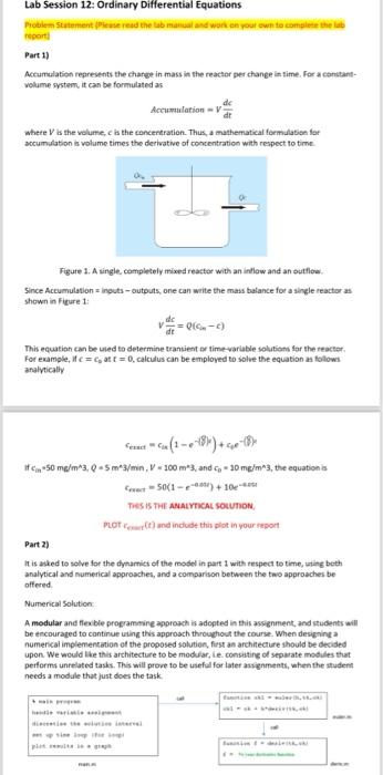

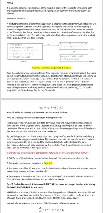
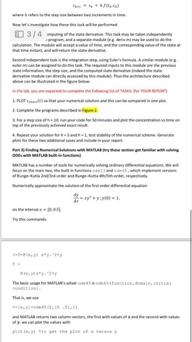
Lab Session 12: Ordinary Differential Equations Problem Stutement (piease resd the lab manual asd won en pour ewn to complete the lab report) Part 1) Accumulation represents the change in mass in the reactor per change in time. For aconstantvolume system, it can be formulated as Accumalation=vdtdc Where V is the volume, c is the concertration. Thus, a mathematical formulation for accumulation is volume times the derivative of concentration with respect to time. Figure 1. A single, completely mixed reactor with an inflow and an butflow. Since Accumulation = incuts - outputs, one can write the mass balance for a slingle reactor as shown in Figure 1 : vdtdc=Q(cinc) This equation can be uled to determine trantient of time-wariable solutions lor the teacter For example, if c=c5 at f=0, calculus can be employed to solve the equation an followi analvically cenact=cin(1e(8))+c4e(8) Ceract=50(1e0.001)+10e406 TReS 15 THE ANALYTACAL SONUTNO. Part 2) It is alked to solve for the dyharnict of the model in part 1 with respect to time, uting beth analytical and numerical approaches, and a comarison between the two approaches be offered. Numerical Solution A modutar and ffex ble programmine approach is adopted in this assignment, and students will be encourated to continue using this approsch throughout the course. When designing a numerical implementation of the proposed solution. fiss an arthifecture should be decided upon. We would the this architecture to be modular, le. consuting of separate modiles that performs unrelated tasks. This will prove to be useful for later assenmenti, when the itudern needs a module that just does the task. Dart 2) If is arsed to solve for the dynarrict of the model in part 1 with respect to time, using beth andytical and numerical approaches, and a comoanion between the two approaches be ctfered. Numerical Solution: A modular and flexble programming approach is adopted in this assignment, and stubents wi be encouraged to continue using this approach throuphout the course. When designing a numerical implementuion of the proposed solution, fint an archsecture phould be decided upon. We would like this arcitecture to be modular, Le, conkating of seowate modules tha performs unvelated tasks. This will prove to be useful for later assignments, when the student reeds a module that just does the task. Figure 2. Schematic diagram of the model Take the architecture proposed in Figure 2 for example, the main proteram (main.m) that takes care of input/output, assionment of variables, discretiuation of solstion imferval, and settine up an incremental wolution wheme (a loop over time that starts fram t=0 to f=tr where tf denotes the final welution time). The presentation of retults in graphical and/or tabulat formats is also done here. Whehin the loop over time inside this main program, certain tasks need to be performed each step, such as calculation of the state derivative, f(t,c), or the integration performed accoidine to Euler's formula. ch+1=cn+hf(c6,cn) where h refers to the step sze betaeen two increments in time. Now let's investigate how these this task wal be performed. Firs consider the computing of the state derivative. Tha task may be taken independently from the rest of the grogram, and a separate module (es. derivim) may be used to do the calculation. The module will actept a value of time, and the coeresponding value of the state at that time instant, and wall returs the state derivative. Second independent takk is the integration step, using Eulet's formula. A simalar module les eulef,m) can be assigred to do this taik. The required inputs to this module tere the previous state information, the step size, and the computed state derivative findeed the state derkative module can directip accessed by this modulel. Thus the arckitecture described above can be iflostated in the ficue below: in the Lab, wou are eapected to complete the following liat ef TNSKS: (for Youm REPOAT) 1. Pior Gmaxr(t) se that your numerical solution and this can be compared in one plot. 2. Complete the programs described in fecure 2 . 3. For a step size of h =10, nun vour code for 50 minutes and plot the concentration vs time on top of the previounly achiewed exact resul. 4. Repeat your solution for h=5 and h=1, test tabaty of the numerical scheme. Generate plots for theie fwo adsitional caies and include is your report. Fart 3) Finding Nureerical Solutions with MATLAB (try these sectien get familiar with solvine oots with MATLAB built-in functions) MaTLAB has a number of tools for numericaly solvine ord nary dfferential equations. We will focus on the main two, the built in functions ode 23 and ode 45 , which implement versions of Runge-Kutsa 2nd/3rd-order and lange-Kuts, Ath/5th-ordet, respectively. Numerically approximate the solution of the first order afferentiat equation dxdy=xy2+y:y(0)=1. cn+1=c2+hf(tk+ck) where ha refers to the step use between two increments in time. Now let's investigate how these this task will be performed. 3/4 imputing of the state derivative. This task may be taken independently a program, and a separate module (e-g-deriv.m) may be used to do the calculation. The module will accept a value of time, and the corresponding value of the state at that time instant, and will return the state derivative. Second independent task is the integration step, using Euler's formula. A similar module fe.e euler.m) can be assigned to do this task. The required inputs to this module are the previous state information, the step size, and the computed state derivative (indeed the state derivative module can directly accessed by this module). Thus the architecture described above can be illustrated in the figure below: In the lab, vou are expected to complete the following lat of TASKS: (for vouR RcpORT) 1. PLot cexart(t) so that your numerical solution and this can be compared in one plot. 2. Complete the programs deseribed in Fleure 2. 3. For a step size of h=10, run your code for 50 minutes and plot the concentration vs time on top of the previously achieved exact result. 4. Repeat your solution for h=5 and h=1, test stability of the numerical scheme. Generate plots for these two additional cases and indlude in your report. Part 3) Finding Numerical Solutions with MATLAE (try these section get familiar with solving OOEs with MATLAB built-in functions) MATLAS has a number of tools for numericaly solving ordinary differential equations. We will focus on the main fwo, the built -in functions ode 23 and odio 45 , which implement versions of Runge-Kutta 2nd/3rd-order and Runge-Kutta 4th/5th-order, respectively. Numerically approximate the solution of the first order differential equation dxdy=xy2+y;y(0)=1. on the interval x={0,05}. Try this commands: x>f=e(x,y)xy,2+yt=(x,y)xy+2+y The bask usage for MATLAB's solver ode45 is ode45 (tunction, doma Lm, in Lt La 1 conditionl. That is, we use (x,y)=code45(f,[0,5],2) and MATLAB returns two column vectors, the first with values of x and the second with values of y, we can plot the values with plot{x,y}itogettheplotofxversusy