Please explain in short summary

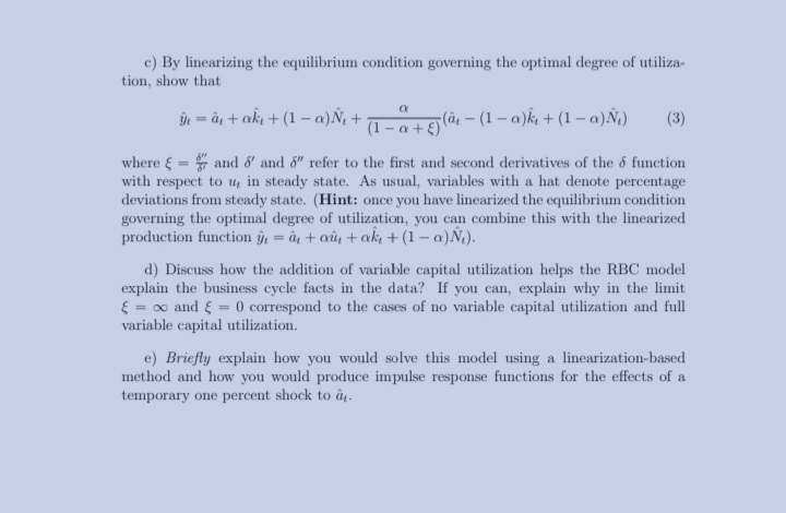
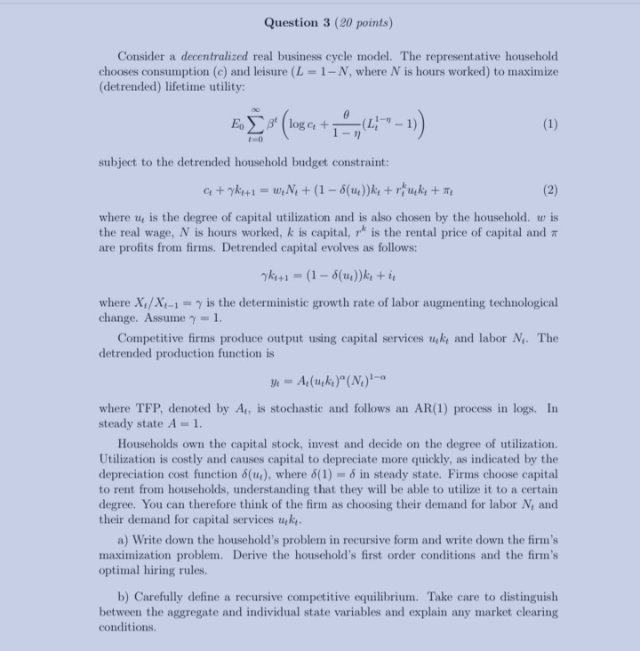
c) By linearizing the equilibrium condition governing the optimal degree of utiliza tion, show that it = an + ake + ( 1 - @ ) Ni+- ( 1 - at E ) (at - (1 - a)k+ (1-a)N.) (3) where { = " and &' and 5" refer to the first and second derivatives of the 6 function with respect to u, in steady state. As usual, variables with a hat denote percentage deviations from steady state. (Hint: once you have linearized the equilibrium condition governing the optimal degree of utilization, you can combine this with the linearized production function y = a + ou tak + (1 - o)N.). d) Discuss how the addition of variable capital utilization helps the RBC model explain the business cycle facts in the data? If you can, explain why in the limit 5 = co and { = 0 correspond to the cases of no variable capital utilization and full variable capital utilization. e) Briefly explain how you would solve this model using a linearization-based method and how you would produce impulse response functions for the effects of a temporary one percent shock to a.Question 3 (20 points) Consider a decentralized real business cycle model. The representative household chooses consumption (c) and leisure (L = 1-N, where N is hours worked) to maximize (detrended) lifetime utility: " EB ( 108a + , ( 1 0 -1)) (1) subject to the detrended household budget constraint: citykiti = wiNet ( 1 - 5( m) )ke + rucke + n (2) where w is the degree of capital utilization and is also chosen by the household. w is the real wage, N is hours worked, & is capital, y is the rental price of capital and T are profits from firms. Detrended capital evolves as follows: Yhit1 = (1 - 8 ( u) )ki tie where Xi/Xi-1 = y is the deterministic growth rate of labor augmenting technological change. Assume y = 1. Competitive firms produce output using capital services uk, and labor M. The detrended production function is 1 = A(ucki )" ( Ni ) 1-a where TFP, denoted by Ar, is stochastic and follows an AR(1) process in logs. In steady state A = 1. Households own the capital stock, invest and decide on the degree of utilization. Utilization is costly and causes capital to depreciate more quickly, as indicated by the depreciation cost function o(us), where o(1) = 6 in steady state. Firms choose capital to rent from households, understanding that they will be able to utilize it to a certain degree. You can therefore think of the firm as choosing their demand for labor N, and their demand for capital services uki. a) Write down the household's problem in recursive form and write down the firm's maximization problem. Derive the household's first order conditions and the firm's optimal hiring rules. b) Carefully define a recursive competitive equilibrium. Take care to distinguish between the aggregate and individual state variables and explain any market clearing conditions.in exchange for go, and let r denote the amount of money the buyer pays in exchange for q1. Describe the bargaining solution in a typical type-j = 0, 1 meeting.? d) Describe the objective function of the typical buyer, J(m'), where the prime denotes next period's choices.3 e) Describe the equilibrium variables go, q1 as functions of the model's parameters, including the nominal interest rate, i. How is q related to the real balances = = om? f) Does a monetary equilibrium (i.e., an equilibrium with > > 0) always exist? If not, describe the set of parameter values (including the policy parameter i) for which such an equilibrium exists. Finally, define the welfare function of this economy as the measure of the various KW market meetings times the net surplus generated in each meeting, i.e., W = olu(go) - go] + (1 - 5)[u(g1) - qi]. g) Can you describe the sign of the term OW/do for the various values of g?4Question 2 (20 points) This question studies the co-existence of money and credit. Time is discrete with an infinite horizon. Each period consists of two subperiods. In the day, trade is partially bilateral and anonymous as in Kiyotaki and Wright (1991) (call this the KW market). At night trade takes place in a Walrasian or centralized market (call this the CM). There are two types of agents, buyers and sellers, and the measure of both is normalized to 1. The per period utility for buyers is u(q) + U(X) - H, and for sellers it is -q + U(X) - H, where q is the quantity of the day good produced by the seller and consumed by the buyer, X is consumption of the night good (the numeraire), and H is hours worked in the CM. In the CM, all agents have access to a technology that turns one unit of work into a unit of good. The functions u, U satisfy the usual assumptions; I will only spell out the most crucial ones: There exists X* E (0, co) such that U'(X*) = 1, and we define the first-best quantity traded in the KW market as q' = {q : u'(q') = 1}. The difference compared to the baseline model is that there are two types of sellers. Type-0 sellers, with measure o E [0, 1), accept credit. More precisely, in meetings with a type-0 seller (type-0 meetings), no medium of exchange (MOE) is necessary, and the buyer can purchase day good by promising to repay the seller in the forthcoming CM with numeraire good (this arrangement is called an IOU). The buyer can promise to repay any amount (no credit limit), and her promise is credible (buyers never default). Type-1 sellers, with measure 1 - o, never accept credit, hence, any purchase of the day good must be paid for on the spot (quid pro quo) with money. All buyers meet a seller in the KW market, so that o is the probability with which a buyer meets a type-0 seller, and 1 - o is the probability with which she meets a type-1 seller. The rest is standard. Goods are non storable. There exits a storable and rec- ognizable object, fiat money, that can serve as a MOE in type-1 meetings. Money supply is controlled by a monetary authority, and we consider simple policies of the form Mil = (1 + #)M, u > 8 -1. New money is introduced, or withdrawn if A 0 per unit of time, and while a firm is searching for a worker it has to pay a search (or recruiting) cost, pe > 0, per unit of time. Firms that are training their workers do not pay this cost (they are done recruiting). Productive jobs are exogenously destroyed at rate > > 0 (only productive jobs are subject to this shock; matches at the training stage cannot be terminated). All agents discount future at the rate r > 0, and unemployed workers enjoy a benefit > > 0 per unit of time. While at the training stage the worker does not receive an unemployment benefit (a trainee is not unemployed). a) Define the value function of the typical firm for all the possible states of the world it may find itself in. b) Do the same for the typical worker. c) Combine the free entry condition with the expressions you provided in part (a) in order to derive the job creation (JC) curve of this economy. d) Using the same methodology as in the lectures (adjusted to accommodate the differences in the new environment), derive the wage curve (WC) for this economy. Hence, two parties who met at time, say, t are negotiating over an object that will be paid in the future (at time t + 1/a, in expected terms). But, as is always the case, the Nash Bargaining problem is to split the generated surplus as of time . 2 e) Provide a restriction on parameter values such that a steady state equilibrium pair (w, 0) exists. Is it unique? (No need for a lengthy discussion.) f) What is the effect of a decrease in a on the equilibrium w and 0? Explain analytically and intuitively (but shortly). g) Describe the Beveridge curve (BC) of this economy by looking at the flows of workers in and out of the various states. What effect will the decrease in a (discussed in the previous part) have on equilibrium unemployment