please give a summary of this article I really need it for a class!!!!!! thank you so much!!!

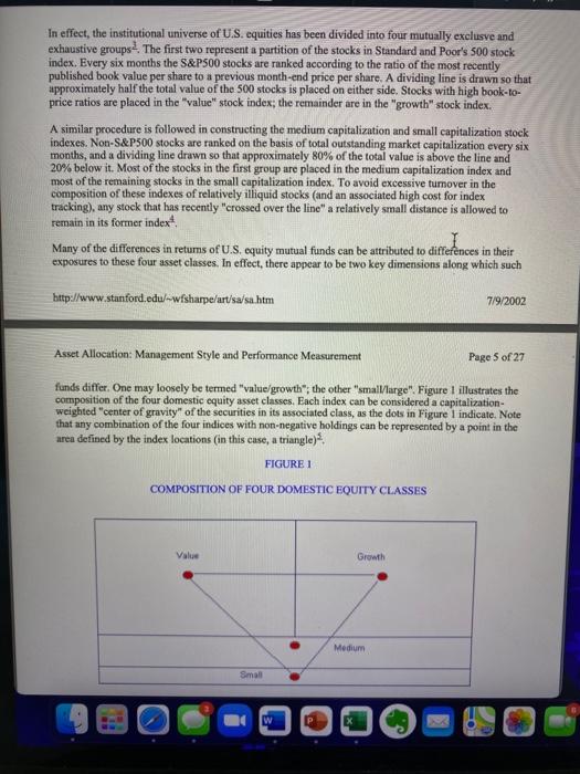
ASSET ALLOCATION: MANAGEMENT STYLE AND PERFORMANCE MEASUREMENT An Asset class factor model can help make order out of chaos William F. Sharpe Reprinted from the Journal of Porffolio Management, Winter 1992, pp. 7-19. o Cagalal CifindaBC, lac. Cenpany. Fhese(2i1) 234-35?. It is widely agreed that asset allocation accounts for a large part of the variability in the return on a typical investor's portfolio. This is especially true if the overall portfolio is invested in multiple funds, each including a number of securities. Asset allocation is generally defined as the allocation of an investor's portfolio among a number of "major" asset classes. Clearly such a generalization cannot be made operational without defining such ciskses. Once a set of asset classes has been defined, it is important to determine the exposures of each component of an investor's overall portfolio to movements in their returns. Such information can be aggregated to determine the investor's overall effective asset mix. If it does not conform to the desired mix, appropriate alterations can then be made. Once a procedure for measuring exposures to variations in returns of major asset classes is in place, it is possible to determine bow effectively individual fuad managers have pefformed their functions and the extent (if any) to which value has been added through active management. Finally, the effectiveness of the invesior's overall asset allocation can be compared with that of one or more benchmark asset mixes. An effective way to accomplish all theie tasks is to use an asset class factor model. After deseribing the characteristics of such a model, we ill astrate applications of a model with twelve asset classes to analyze the performance of a set of open-end mutual funds between 1985 and 1989. ASSET CLASS FACTOR MODELS Factor models aire common in investment analysis. Fquation (1) is a generie repersentation: R3=[b1R1+b2F2++bnFm]+z1 Fi, represchts the feium oe assef 1,Fi represents the value of factor 1,Fi2 the value of factor 2,Fin the value of the n'th (last) factor and ej the "non-factor" component of the retum on i. All these values are (potentially) unknown before-the-fact, as indicated by the tildes. The remaining values (b, through bin) represent the sensitivities of Ri to factors Fi1 through Fin. A key assumption makes a model of this sort more than simply an exercise in data description: The nonfactor retum for one asset (ei) is assumed to be uncorrelated with that of every other (ege). In effeet, the factors are the only sources of correlation among returns. An asset class factor model can be considered a special case of the gencric type. In such a model each factor represents the return on an asset class and the sensitivities (bij values) are required to sum to 1 (100\%). In effect, the return on an asset i is represented as the return on a portfolio (shown by the sum of the terms in the bracketed expression) invested in the n asset classes plus a residual component (ej). For expository convenience, the sum of the terms in the brackets can be termed the return attributable to style and the residual component (j) the retum due to selection. Indeed, a key contributibn of this approsch is the separation of return into these two main components. EVALUATING ASSET CLASS FACTOR MODELS The usefulness of an asset class factor model depends on the asset classes chosen for its implementation. While not strietly necessary, it is desirable that such asset classes be I) matually exclusive, 2) exhaustive and 3) have retums that "differ", Pragmatically, each should represeat a market-capitalization weighted portfolio of securities; no security should be included in more than one asset class; as many securities as possible should be included in the chosen asset classe; and the asset class returns should either have low correlations with one another or, in cases in which correlations are high, different standard deviations. While the appropriate messure of the efficacy of any specific implementation depends on the uses to which the model is to be put, factor models are typically evaluated on the basis of their ability to explain the returns of the assets in question (L.e. the Rj ). A useful metric is the proportion of variance "explained" by the selected asset classes. Using the traditional definition, for asset i: R21Var(1R)Var(1) The right-hand side of equation (2) equals 1 minus the proportion of variance "uncexplained". The resulting R-squared value thus indicates the proportion of the variance of Ri "explained" by the n asset classest. It is important to recognize that this measure indicates only the extent to which a specific model fits the data at bund. A better test of the usefalness of any implementation is its ability to explain performance out-of-sample. For this reason it is important to consider not only the ability of a model to explais a given set of data but also its parnimony. Other things cqual (c.g. R-squared values), the fewer the asset classes, the more likely is the model to represent continuing fundamental relationships with predistive bttp://www,stanford.edw-wfsharpe/ar//sa/sa hitm 7992002 Asset Allocation: Management Style and Performance Measurement Page 3 of 27 content 2 To evaluate the exposures of funds to changes in the returns of key asset classes, the appropriate measure is the collective ability of a set of such classes to explain the time-series variability in the returns on a typical fund (e.g. mutual fund or separately-managed institutional account). Note that this criterion differs from that often applied in evaluating factor models designed to describe specific portions of the overall capital market. For example, when constructing an equity factor model, one might consider the ability of the selected factors to explain the time-series variation in the returns of a typical stock. Most stock market models include factors representing returns on industry groups and/or economic sectors - factors that account for much of the typical security's return. If most managers diversify across industries anc economic sectors, however, inclusion of factors related to differences in industry and sector returns will add little if any explanatory power to a model designed to explain fund returns. A TWELVE ASSET CLASS MODEL The model we use has twelve asset classes. The retum of each is represented by a market capitalization weighted index of the returns on a large number of securities. For reasons that will become clear, it is important to note that each index represents a strategy that could be followed at low cost using an index fund. The composition of each index is specified in sufficient detail by its provider to enable an investor to track the returns with little error through a passive (index-like) investment strategy. Table 1 describes the twelve asset classes and the indices used for the associated return series. Most are widely used indexes that require no further description. The four less well-known are those employed to represent U.S. equity classes. In effect, the institutional universe of U.S. equities has been divided into four mutually exclusve and exhaustive groups 2. The first two represent a partition of the stocks in Standard and Poor's 500 stock index. Every six months the S\&PS00 stocks are ranked according to the ratio of the most recently published book value per share to a previous month-end price per share. A dividing line is drawn so that approximately half the total value of the 500 stocks is placed on either side. Stocks with high book-loprice ratios are placed in the "value" stock index; the remainder are in the "growth" stock index. A similar procedure is followed in constructing the medium capitalization and small capitalization stock indexes. Non-S\&P500 stocks are ranked on the basis of total outstanding market capitalization every six months, and a dividing line drawn so that approximately 80% of the total value is above the line and 20% below it. Most of the stocks in the first group are placed in the medium capitalization index and most of the remaining stocks in the small capitalization index. To avoid excessive tumover in the composition of these indexes of relatively illiquid stocks (and an associated high cost for index tracking), any stock that has recently "crossed over the line" a relatively small distance is allowed to remain in its former index x4, Many of the differenees in retums of U.S. equity mutual funds can be attributed to differences in their exposures to these four asset classes. In effect, there appear to be two key dimensions along which such bttp://www.stanford.edu/-wfshame/art/sa/sa htm 7/9/2002 Asset Allocation: Management Style and Performance Measurement Page 5 of 27 funds differ, One may loosely be termed "value/growth"; the other "small/arge". Figure 1 illustrates the composition of the four domestic equity asset classes, Each index can be considered a capitalizationweighted "center of gravity" of the securities in its associated class, as the dots in Figure I indicate. Note that any combination of the four indices with non-negative holdings can be represented by a point in the area deIined by the index locations (in this case, a triangle) 2. FIGURE 1 COMPOSITION OF FOUR DOMESTIC EQUTTY CLASSES Much has been written about both the small-stock and the valuedgrowth phenomena. While the terms "value" and "growth" reflect common usage in the investment profession, they serve only as convenient names for stocks that tend to be similar in several respects. As is well known, across securities there is significant positive correlation among: book/price, earnings/price, low earnings growth, dividend yield and low return on equity. Moreover, the industry compositions of the value and growth groups differ (e.g. companies with high research budgets tend to have low book values relative to their stock prices). Those concemed with these distinctions have focused most of their research on long-run average return differences; that is, they have asked whether small stocks or value stocks "do better than they should" in the long-run. Less attention has been paid to likely sources of short-run variability in returns among such groups. For present purposes it suffices that such variability is substantial. Figure 2 provides relevant evidence: The variability in returns across the four asset classes from year-toyear is far greater than would be encountered if groups with similar numbers of securities had been formed randomly. Fund exposures across these dimensions vary greatly. As a result, muph of the variation in fund returns in any given period can be attributed to the combined effects of their exposures to these asset classes and the realized retums on those classes. http://ww.stanford.edu/-wfsharpe/art/sa/sa.htm 7/9/2002 Asset Allocation: Management Style and Performance Measurement Page 6 of 27 DETERMINING FUND EXPOSURES The traditional view of asset allocation assumes that an investor allocates assets among (potentially many) funds, each of which holds (potentially many) securities. Ultimately one is interested in the investor's exposures to the key asset classes. These are a function of 1) the amounts of the investor's portfolio invested in the various funds and 2) the exposures of each such fund to the asset classes. The exposures of a fund to the various asset classes are, in tum, a function of 1 ) the amounts that the fund has invested in various securities and 2) the exposures of the securities to the asset classes. While it is possible to attempt to determine a fund's exposures from a detailed analysis of the securities held by the fund, a simpler approach typically provides more than enough information for purposes of asset allocation. Such a method uses only realized fund returns to infer the typical exposures of the fund to the asset classes. Since only easily obtained information is required, the approach may be considered "external", in comparison with methods that rely on information that may be available only from sources internal to the fund. Inspection of equation (1) immediately suggests a procedure that might be used in this connection. Given, say, sixty monthly returns on a fund, along with comparable returns for a selected set of asset classes, one could simply employ a multiple regression analysis with fund retums as the dependent variable and asset class returns as the independent variables. The resulting slope coefficients could then be intererpreted as the fund's historic exposures to the asset class retums. Table 2 provides an example for Trustees' Commingled U.S. Portfolio (an open-end mutual fund offered by the Vanguard Group). Monthly returns from January 1985 through Decenber 1989 are used for the dependent variable, with the corresponding returns for the twelve asset classes serving as independent variables. The column entitled "Unconstrained Regression" shows results obtained applying Equation (1). The first twelve rows show the resulting slope coefficients ( bij values), expressed as percentages. The coefficient total is shown next, followed by the R-squared value (also expressed as a percentage). A substantial portion (95.20% ) of the monthly variance in the fund's returns is explained by this equation. The htti://www.stanford.edu/-wfsharpe/art/sa/sa.htm 7/9/2002 Asset Allocation: Management Style and Performance Measurement Page 7 of 27 coefficients, however, do not sum to 100%. What is more important, several are vastly inconsistent with the fund's actual policy (to invest in common stocks with no short positions). ASSET ALLOCATION: MANAGEMENT STYLE AND PERFORMANCE MEASUREMENT An Asset class factor model can help make order out of chaos William F. Sharpe Reprinted from the Journal of Porffolio Management, Winter 1992, pp. 7-19. o Cagalal CifindaBC, lac. Cenpany. Fhese(2i1) 234-35?. It is widely agreed that asset allocation accounts for a large part of the variability in the return on a typical investor's portfolio. This is especially true if the overall portfolio is invested in multiple funds, each including a number of securities. Asset allocation is generally defined as the allocation of an investor's portfolio among a number of "major" asset classes. Clearly such a generalization cannot be made operational without defining such ciskses. Once a set of asset classes has been defined, it is important to determine the exposures of each component of an investor's overall portfolio to movements in their returns. Such information can be aggregated to determine the investor's overall effective asset mix. If it does not conform to the desired mix, appropriate alterations can then be made. Once a procedure for measuring exposures to variations in returns of major asset classes is in place, it is possible to determine bow effectively individual fuad managers have pefformed their functions and the extent (if any) to which value has been added through active management. Finally, the effectiveness of the invesior's overall asset allocation can be compared with that of one or more benchmark asset mixes. An effective way to accomplish all theie tasks is to use an asset class factor model. After deseribing the characteristics of such a model, we ill astrate applications of a model with twelve asset classes to analyze the performance of a set of open-end mutual funds between 1985 and 1989. ASSET CLASS FACTOR MODELS Factor models aire common in investment analysis. Fquation (1) is a generie repersentation: R3=[b1R1+b2F2++bnFm]+z1 Fi, represchts the feium oe assef 1,Fi represents the value of factor 1,Fi2 the value of factor 2,Fin the value of the n'th (last) factor and ej the "non-factor" component of the retum on i. All these values are (potentially) unknown before-the-fact, as indicated by the tildes. The remaining values (b, through bin) represent the sensitivities of Ri to factors Fi1 through Fin. A key assumption makes a model of this sort more than simply an exercise in data description: The nonfactor retum for one asset (ei) is assumed to be uncorrelated with that of every other (ege). In effeet, the factors are the only sources of correlation among returns. An asset class factor model can be considered a special case of the gencric type. In such a model each factor represents the return on an asset class and the sensitivities (bij values) are required to sum to 1 (100\%). In effect, the return on an asset i is represented as the return on a portfolio (shown by the sum of the terms in the bracketed expression) invested in the n asset classes plus a residual component (ej). For expository convenience, the sum of the terms in the brackets can be termed the return attributable to style and the residual component (j) the retum due to selection. Indeed, a key contributibn of this approsch is the separation of return into these two main components. EVALUATING ASSET CLASS FACTOR MODELS The usefulness of an asset class factor model depends on the asset classes chosen for its implementation. While not strietly necessary, it is desirable that such asset classes be I) matually exclusive, 2) exhaustive and 3) have retums that "differ", Pragmatically, each should represeat a market-capitalization weighted portfolio of securities; no security should be included in more than one asset class; as many securities as possible should be included in the chosen asset classe; and the asset class returns should either have low correlations with one another or, in cases in which correlations are high, different standard deviations. While the appropriate messure of the efficacy of any specific implementation depends on the uses to which the model is to be put, factor models are typically evaluated on the basis of their ability to explain the returns of the assets in question (L.e. the Rj ). A useful metric is the proportion of variance "explained" by the selected asset classes. Using the traditional definition, for asset i: R21Var(1R)Var(1) The right-hand side of equation (2) equals 1 minus the proportion of variance "uncexplained". The resulting R-squared value thus indicates the proportion of the variance of Ri "explained" by the n asset classest. It is important to recognize that this measure indicates only the extent to which a specific model fits the data at bund. A better test of the usefalness of any implementation is its ability to explain performance out-of-sample. For this reason it is important to consider not only the ability of a model to explais a given set of data but also its parnimony. Other things cqual (c.g. R-squared values), the fewer the asset classes, the more likely is the model to represent continuing fundamental relationships with predistive bttp://www,stanford.edw-wfsharpe/ar//sa/sa hitm 7992002 Asset Allocation: Management Style and Performance Measurement Page 3 of 27 content 2 To evaluate the exposures of funds to changes in the returns of key asset classes, the appropriate measure is the collective ability of a set of such classes to explain the time-series variability in the returns on a typical fund (e.g. mutual fund or separately-managed institutional account). Note that this criterion differs from that often applied in evaluating factor models designed to describe specific portions of the overall capital market. For example, when constructing an equity factor model, one might consider the ability of the selected factors to explain the time-series variation in the returns of a typical stock. Most stock market models include factors representing returns on industry groups and/or economic sectors - factors that account for much of the typical security's return. If most managers diversify across industries anc economic sectors, however, inclusion of factors related to differences in industry and sector returns will add little if any explanatory power to a model designed to explain fund returns. A TWELVE ASSET CLASS MODEL The model we use has twelve asset classes. The retum of each is represented by a market capitalization weighted index of the returns on a large number of securities. For reasons that will become clear, it is important to note that each index represents a strategy that could be followed at low cost using an index fund. The composition of each index is specified in sufficient detail by its provider to enable an investor to track the returns with little error through a passive (index-like) investment strategy. Table 1 describes the twelve asset classes and the indices used for the associated return series. Most are widely used indexes that require no further description. The four less well-known are those employed to represent U.S. equity classes. In effect, the institutional universe of U.S. equities has been divided into four mutually exclusve and exhaustive groups 2. The first two represent a partition of the stocks in Standard and Poor's 500 stock index. Every six months the S\&PS00 stocks are ranked according to the ratio of the most recently published book value per share to a previous month-end price per share. A dividing line is drawn so that approximately half the total value of the 500 stocks is placed on either side. Stocks with high book-loprice ratios are placed in the "value" stock index; the remainder are in the "growth" stock index. A similar procedure is followed in constructing the medium capitalization and small capitalization stock indexes. Non-S\&P500 stocks are ranked on the basis of total outstanding market capitalization every six months, and a dividing line drawn so that approximately 80% of the total value is above the line and 20% below it. Most of the stocks in the first group are placed in the medium capitalization index and most of the remaining stocks in the small capitalization index. To avoid excessive tumover in the composition of these indexes of relatively illiquid stocks (and an associated high cost for index tracking), any stock that has recently "crossed over the line" a relatively small distance is allowed to remain in its former index x4, Many of the differenees in retums of U.S. equity mutual funds can be attributed to differences in their exposures to these four asset classes. In effect, there appear to be two key dimensions along which such bttp://www.stanford.edu/-wfshame/art/sa/sa htm 7/9/2002 Asset Allocation: Management Style and Performance Measurement Page 5 of 27 funds differ, One may loosely be termed "value/growth"; the other "small/arge". Figure 1 illustrates the composition of the four domestic equity asset classes, Each index can be considered a capitalizationweighted "center of gravity" of the securities in its associated class, as the dots in Figure I indicate. Note that any combination of the four indices with non-negative holdings can be represented by a point in the area deIined by the index locations (in this case, a triangle) 2. FIGURE 1 COMPOSITION OF FOUR DOMESTIC EQUTTY CLASSES Much has been written about both the small-stock and the valuedgrowth phenomena. While the terms "value" and "growth" reflect common usage in the investment profession, they serve only as convenient names for stocks that tend to be similar in several respects. As is well known, across securities there is significant positive correlation among: book/price, earnings/price, low earnings growth, dividend yield and low return on equity. Moreover, the industry compositions of the value and growth groups differ (e.g. companies with high research budgets tend to have low book values relative to their stock prices). Those concemed with these distinctions have focused most of their research on long-run average return differences; that is, they have asked whether small stocks or value stocks "do better than they should" in the long-run. Less attention has been paid to likely sources of short-run variability in returns among such groups. For present purposes it suffices that such variability is substantial. Figure 2 provides relevant evidence: The variability in returns across the four asset classes from year-toyear is far greater than would be encountered if groups with similar numbers of securities had been formed randomly. Fund exposures across these dimensions vary greatly. As a result, muph of the variation in fund returns in any given period can be attributed to the combined effects of their exposures to these asset classes and the realized retums on those classes. http://ww.stanford.edu/-wfsharpe/art/sa/sa.htm 7/9/2002 Asset Allocation: Management Style and Performance Measurement Page 6 of 27 DETERMINING FUND EXPOSURES The traditional view of asset allocation assumes that an investor allocates assets among (potentially many) funds, each of which holds (potentially many) securities. Ultimately one is interested in the investor's exposures to the key asset classes. These are a function of 1) the amounts of the investor's portfolio invested in the various funds and 2) the exposures of each such fund to the asset classes. The exposures of a fund to the various asset classes are, in tum, a function of 1 ) the amounts that the fund has invested in various securities and 2) the exposures of the securities to the asset classes. While it is possible to attempt to determine a fund's exposures from a detailed analysis of the securities held by the fund, a simpler approach typically provides more than enough information for purposes of asset allocation. Such a method uses only realized fund returns to infer the typical exposures of the fund to the asset classes. Since only easily obtained information is required, the approach may be considered "external", in comparison with methods that rely on information that may be available only from sources internal to the fund. Inspection of equation (1) immediately suggests a procedure that might be used in this connection. Given, say, sixty monthly returns on a fund, along with comparable returns for a selected set of asset classes, one could simply employ a multiple regression analysis with fund retums as the dependent variable and asset class returns as the independent variables. The resulting slope coefficients could then be intererpreted as the fund's historic exposures to the asset class retums. Table 2 provides an example for Trustees' Commingled U.S. Portfolio (an open-end mutual fund offered by the Vanguard Group). Monthly returns from January 1985 through Decenber 1989 are used for the dependent variable, with the corresponding returns for the twelve asset classes serving as independent variables. The column entitled "Unconstrained Regression" shows results obtained applying Equation (1). The first twelve rows show the resulting slope coefficients ( bij values), expressed as percentages. The coefficient total is shown next, followed by the R-squared value (also expressed as a percentage). A substantial portion (95.20% ) of the monthly variance in the fund's returns is explained by this equation. The htti://www.stanford.edu/-wfsharpe/art/sa/sa.htm 7/9/2002 Asset Allocation: Management Style and Performance Measurement Page 7 of 27 coefficients, however, do not sum to 100%. What is more important, several are vastly inconsistent with the fund's actual policy (to invest in common stocks with no short positions)