Please give correct explanation thankyou

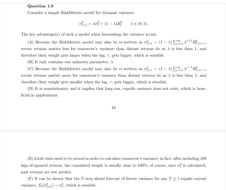
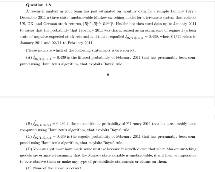
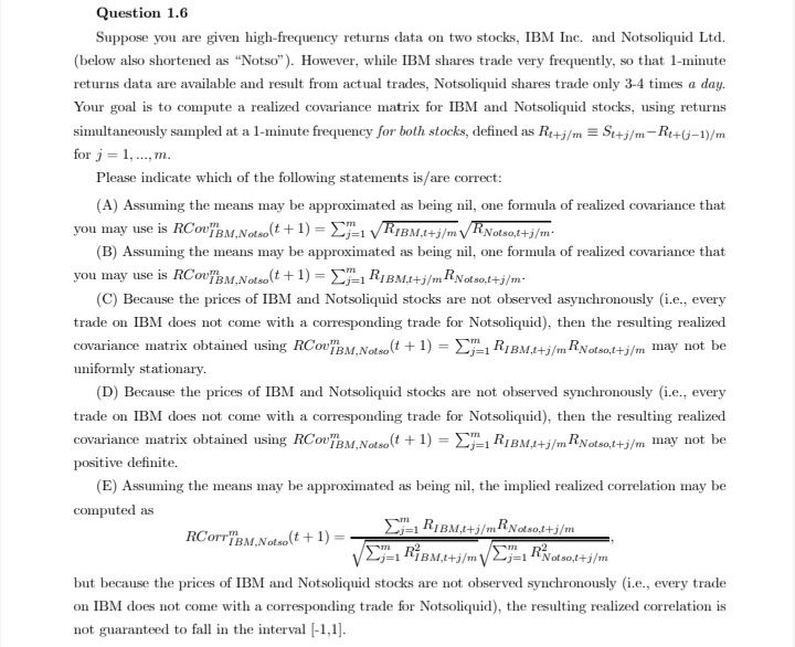
Question 2.1 You are asked to construct a portfolio by using 5 electronically traded funds (ETFs) that replicate the indexes of the US, Japan, UK, Euro area, and the Brazilian stock markets. Your benchmark for evaluating the resulting portfolio is the MSCI world index. You have to choose the optimal weights to maximize the Sharpe ratio of your portfolio with an investing horizon of three years. Given your choice of the weights in your portfolio, you should then compute the daily, weekly and monthly 1 percent value Value-at-Risk (VaR) of your portfolio. You have access to 30 years of data on the fundamentals (the earning/price and the dividend price ratios) underlying stock index prices and to returns on the relevant ETFs, all at daily frequencies (and therefore at any frequency lower than the daily one). Answer the following questions justifying your answers. 2.1(a) Explain how you would proceed to construct your portfolio. State all the assumptions that you think are appropriate.Question 1.9 Consider a simple RiskMetrics model for dynamic variance: 0141 = 207 + (1 - A)R; AE (0,1). The key advantage(s) of such a model when forecasting the variance is/are: (A) Because the RiskMetrics model may also be re-written as off = (1 - A) ER, At Ritter, recent returns matter less for tomorrow's variance than distant returns do as A is less than 1, and therefore their weight gets larger when the lag, 7, gets bigger, which is sensible. (B) It only contains one unknown parameter, A. (C) Because the RiskMetrics model may also be re-written as off = (1 - A), ) Ritz-,, recent returns matter more for tomorrow's variance than distant returns do as A is less than 1, and therefore their weight gets smaller when the lag, T, gets bigger, which is sensible. (D) It is nonstationary and it implies that long-run, ergodic variance does not exist, which is bene- ficial in applications. 10 (E) Little data need to be stored in order to calculate tomorrow's variance; in fact, after including 100 lags of squared returns, the cumulated weight is usually close to 100%; of course, once of is calculated, past returns are not needed. (F) It can be shown that the T'-step ahead forecast of future variance for any 7 2 1 equals current variance, Erof+p] = 07, which is sensible.Question 1.8 A research analyst in your team has just estimated on monthly data for a sample January 1972 - December 2011 a three-state, unobservable Markov switching model for a trivariate system that collects US, UK, and German stock returns, [RYS RYK RSer]'. He/she has then used data up to January 2011 to assess that the probability that February 2011 was characterized as an occurrence of regime 1 (a bear state of negative expected stock returns) and that it equalled 502/1101/11 = 0.439, where 01/11 refers to January 2011 and 02/11 to February 2011. Please indicate which of the following statements is/are correct: (A) 502/1101/11 = 0.439 is the filtered probability of February 2011 that has presumably been com- puted using Hamilton's algorithm, that exploits Bayes' rule. (B) 502/1101/11 = 0.439 is the unconditional probability of February 2011 that has presumably been computed using Hamilton's algorithm, that exploits Bayes' rule. (C) 502/1101/11 = 0.439 is the ergodic probability of February 2011 that has presumably been com- puted using Hamilton's algorithm, that exploits Bayes' rule. (D) Your analyst must have made some mistake because it is well-known that when Markov switching models are estimated assuming that the Markov state variable is unobservable, it will then be impossible to ever observe them or make any type of probabilistic statements or claims on them. (E) None of the above is correct.Question 1.6 Suppose you are given high-frequency returns data on two stocks, IBM Inc. and Notsoliquid Ltd. (below also shortened as "Notso"). However, while IBM shares trade very frequently, so that 1-minute returns data are available and result from actual trades, Notsoliquid shares trade only 3-4 times a day. Your goal is to compute a realized covariance matrix for IBM and Notsoliquid stocks, using returns simultaneously sampled at a 1-minute frequency for both stocks, defined as Rij/m = St+j/m -Re+(-1)/m for j = 1, ..., m. Please indicate which of the following statements is/are correct: (A) Assuming the means may be approximated as being nil, one formula of realized covariance that you may use is RCOv"BM,Notso(t + 1) = 2;=1 VRIBM,t+j/mVRNotso,t+j/m. (B) Assuming the means may be approximated as being nil, one formula of realized covariance that you may use is RCOv"BM,Notso(t + 1) = Ejt RIBMIti/mNotsol+j/m- (C) Because the prices of IBM and Notsoliquid stocks are not observed asynchronously (i.e., every trade on IBM does not come with a corresponding trade for Notsoliquid), then the resulting realized covariance matrix obtained using RCOv"By,Notso(1 + 1) = 212 RIBM.1+j/mRNotsoftj/m may not be uniformly stationary. (D) Because the prices of IBM and Notsoliquid stocks are not observed synchronously (i.e., every trade on IBM does not come with a corresponding trade for Notsoliquid), then the resulting realized covariance matrix obtained using RCOv"BM,Notso( + 1) = 2;2, RIBM.:4j/m RNotsoftj/m may not be positive definite. (E) Assuming the means may be approximated as being nil, the implied realized correlation may be computed as RCOTT TEM,Notso(t + 1) =- 21= RIBMIti/mNotsot+j/m VEJ-, RiBM,tti/m \\EJ=1 RNatsotti/m but because the prices of IBM and Notsoliquid stocks are not observed synchronously (i.e., every trade on IBM does not come with a corresponding trade for Notsoliquid), the resulting realized correlation is not guaranteed to fall in the interval [-1,1].Question 1.5 You have just given a presentation to the board of directors of your institution in which you have presented results for a number of predicted, back-tested (i.e., recursively computed over time) VaR mea- sures (with their level p set to range between 1 and 20%) for the overall portfolio held by your institution, over a 10-year period. Such recursive VaR measures have been computed under five alternative models: (i) a naive, homoskedastic Gaussian IID model with zero mean returns; (ii) a plain-vanilla Gaussian GARCH(1,1) model with zero mean returns; (ii) a plain-vanilla Gaussian GARCH(1,1) model with estimated mean returns, ; (iv) a t-Student GARCH(1,1) model with estimated mean returns, ; (v) a DCC-GARCH(1,1) model estimated for the vector of returns on the main asset classes in the portfolio of your bank. Note that models (i)-(iv) are estimated directly on the series of portfolio returns, i.e., these are passive risk management models, while (v) may be implemented as an active model. A colleague of yours has criticized your results and in particular he/she has pointed out three alleged inconsistencies that would affect your simulations/backtesting exercises: -1- There are long time periods in which the Gaussian IID VaR [model (i)] exceeds the VaR yielded by the other models [(ii)-(v)] and this cannot be, because (so he/she says) we all know that fancier and more complex econometric models ought to make us always more prudent in risk management terms. -2- There are time periods in which the t-Student GARCH(1,1) [model (iv)] yields VaR measures that fail to exceed the Gaussian GARCH(1,1) measures [model (iii)] and this cannot be, because (so he/she says) we all know that modelling shocks as t-Student shocks cannot but increase VaR, thus making us more prudent. -3- There are time periods in which the plain-vanilla GARCH(1,1) model with zero mean returns [model (ii)] yields VaR measures exceeding the Gaussian GARCH(1,1) measures with estimated mean [model (iii)] and this cannot be, because (so he/she says) we all know that imposing a zero mean will always reduce VaR measures, thus making us less prudent. 5 Your colleague asks that you be fired: on which counts is she correct, if any? (A) 1 only. (B) 1 and 3. (C) 2 and 3. (D) 3 only. (E) 1 and 2. (F) None