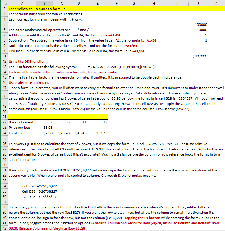
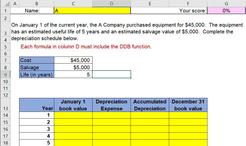
Please help!

D E F A B F G H J K 2 Each yellow cell requires a formula. 3. The formula must only contain cell addresses. 4 Each correct formula will begin with 5, +, or 5 100000 6 The basic mathematical operators are +,, * and/ 10000 7 Addition: To add the values in cells A1 and B4, the formula is =A1+B4 5 8 Subtraction: To subtract the value in cell B4 from the value in cell A1, the formula is =A1-B4 1 9 Multiplication: To multiply the values in cells A1 and B4, the formula is =A1*B4 10 Division: To divide the value in cell A1 by the value in cell B4, the formula is =A1/B4 11 $40,000 12 Using the DDB function 13 The DDB function has the following syntax: -SLN(COST,SALVAGE,LIFE,PERIOD, (FACTOR]) 14 Each variable may be either a value or a formula that returns a value. 15 The final variable, factor, is the depreciation rate. If omitted, it is presumed to be double declining balance. 16 Using absolute addresses 17 Once a formula is created, you will often want to copy the formula to other columns and rows. It's important to understand that excel always uses "relative addresses" unless you indicate otherwise by creating an "absolute address". For example, if you are 18 calculating the cost of purchasing 2 boxes of cereal at a cost of $3.95 per box, the formula in cell B28 is =B26*B27. Although we read cell B28 as "Multiply 2 boxes by $3.95", Excel is actually calculating the value in cell B28 as "Multiply the value in the cell in the 19 same column (column B) 2 rows above (row 26) by the value in the cell in the same column 1 row above (row 27). 20 21 22 Boxes of cereal 11 15 23 Price per box $3.95 24 Total cost $7.90 $23.70 $43.45 $59.25 25 26 This works just fine to calculate the cost of 2 boxes, but if we copy the formula in cell B28 to C28, Excel will assume relative 27 references. The formula in cell C28 will become =C26*c27. Since Cell C27 is blank, the formula will return a value of $0 (which is an 28 excellent deal for 6 boxes of cereal, but it isn't accurate!) Adding a $sign before the column or row reference locks the formula to a 29 specific location. 30 31 If we modify the formula in cell B28 to =B26*$B$27 before we copy the formula, Excel will not change the row or the column of the 32 second variable. When the formula is copied to columns C through E, the formulas become: 33 Cell C28 =C26*$B$27 35 Cell D28 =D26*$B$27 36 Cell E28 =E26*$B$27 37 38 Sometimes, you will want the column to stay fixed, but allow the row to remain relative when it's copied. If so, add a dollar sign 39 before the column, but not the row (i.e.$B27) If you want the row to stay fixed, but allow the column to remain relative when it's 40 copied, add a dollar sign before the row, but not the column (i.e. B$27). Tapping the F4 button while entering the formula (or in the 41 formula bar) toggles among the 3 absolute options (Absolute Column and Absolute Row $B$28, Absolute Column and Relative Row 42 SB28, Relative Column and Absolute Row B$28) 2 6 34 A B E G F Your score: 1 Name: | 0% 2 On January 1 of the current year, the A Company purchased equipment for $45,000. The equipment 3 has an estimated useful life of 5 years and an estimated salvage value of $5,000. Complete the 4 depreciation schedule below. 5 Each formula in column D must include the DDB function. 6 7 Cost $45,000 8 Salvage $5,000 Life (in years) 5 10 9 11 12 January 1 book value Depreciation Expense Accumulated December 31 Depreciation book value 13 Year 1 2 3 15 16 17 18 4 5 D E F A B F G H J K 2 Each yellow cell requires a formula. 3. The formula must only contain cell addresses. 4 Each correct formula will begin with 5, +, or 5 100000 6 The basic mathematical operators are +,, * and/ 10000 7 Addition: To add the values in cells A1 and B4, the formula is =A1+B4 5 8 Subtraction: To subtract the value in cell B4 from the value in cell A1, the formula is =A1-B4 1 9 Multiplication: To multiply the values in cells A1 and B4, the formula is =A1*B4 10 Division: To divide the value in cell A1 by the value in cell B4, the formula is =A1/B4 11 $40,000 12 Using the DDB function 13 The DDB function has the following syntax: -SLN(COST,SALVAGE,LIFE,PERIOD, (FACTOR]) 14 Each variable may be either a value or a formula that returns a value. 15 The final variable, factor, is the depreciation rate. If omitted, it is presumed to be double declining balance. 16 Using absolute addresses 17 Once a formula is created, you will often want to copy the formula to other columns and rows. It's important to understand that excel always uses "relative addresses" unless you indicate otherwise by creating an "absolute address". For example, if you are 18 calculating the cost of purchasing 2 boxes of cereal at a cost of $3.95 per box, the formula in cell B28 is =B26*B27. Although we read cell B28 as "Multiply 2 boxes by $3.95", Excel is actually calculating the value in cell B28 as "Multiply the value in the cell in the 19 same column (column B) 2 rows above (row 26) by the value in the cell in the same column 1 row above (row 27). 20 21 22 Boxes of cereal 11 15 23 Price per box $3.95 24 Total cost $7.90 $23.70 $43.45 $59.25 25 26 This works just fine to calculate the cost of 2 boxes, but if we copy the formula in cell B28 to C28, Excel will assume relative 27 references. The formula in cell C28 will become =C26*c27. Since Cell C27 is blank, the formula will return a value of $0 (which is an 28 excellent deal for 6 boxes of cereal, but it isn't accurate!) Adding a $sign before the column or row reference locks the formula to a 29 specific location. 30 31 If we modify the formula in cell B28 to =B26*$B$27 before we copy the formula, Excel will not change the row or the column of the 32 second variable. When the formula is copied to columns C through E, the formulas become: 33 Cell C28 =C26*$B$27 35 Cell D28 =D26*$B$27 36 Cell E28 =E26*$B$27 37 38 Sometimes, you will want the column to stay fixed, but allow the row to remain relative when it's copied. If so, add a dollar sign 39 before the column, but not the row (i.e.$B27) If you want the row to stay fixed, but allow the column to remain relative when it's 40 copied, add a dollar sign before the row, but not the column (i.e. B$27). Tapping the F4 button while entering the formula (or in the 41 formula bar) toggles among the 3 absolute options (Absolute Column and Absolute Row $B$28, Absolute Column and Relative Row 42 SB28, Relative Column and Absolute Row B$28) 2 6 34 A B E G F Your score: 1 Name: | 0% 2 On January 1 of the current year, the A Company purchased equipment for $45,000. The equipment 3 has an estimated useful life of 5 years and an estimated salvage value of $5,000. Complete the 4 depreciation schedule below. 5 Each formula in column D must include the DDB function. 6 7 Cost $45,000 8 Salvage $5,000 Life (in years) 5 10 9 11 12 January 1 book value Depreciation Expense Accumulated December 31 Depreciation book value 13 Year 1 2 3 15 16 17 18 4 5