please help

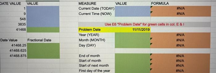
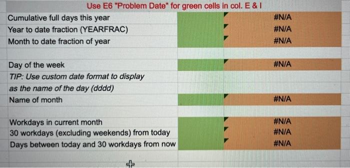
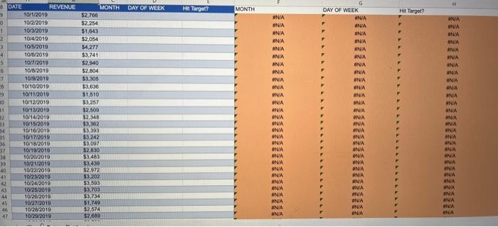
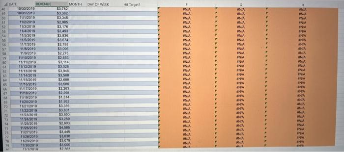
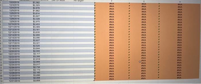
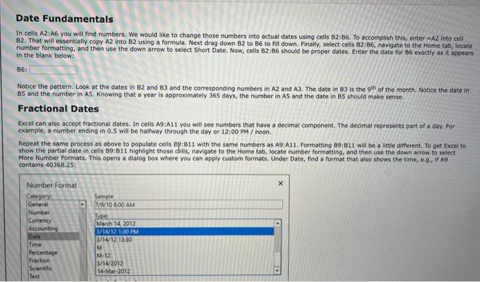
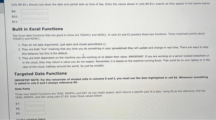
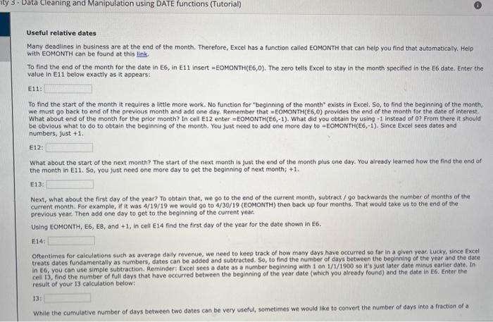
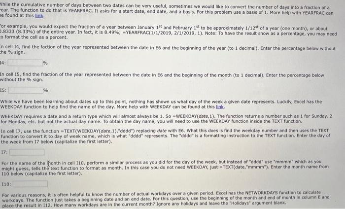
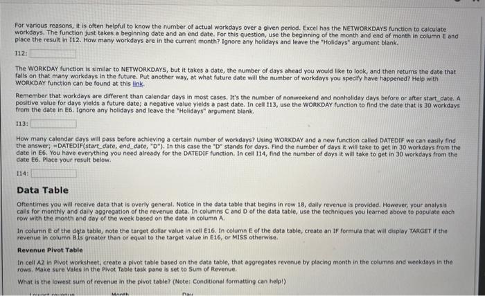
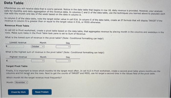
DATE VALUE VALUE MEASURECurrentDate(TODAY)CurrentTime(NOW)VALUE#N/AFORMULA#N/A Use E6 "Problem Date" for green cells in col. E \& I 11/11/2019 Problem Date Year (YEAR) Month (MONTH) \#N/A Date Value 41468.25 Day (DAY) \#N/A \#N/A 41468.625 End of month Start of month Start of next month First day of the year \#N/A \#N/A \#N/A \#N/A Use E6 "Problem Date" for green cells in col. E \& I Cumulative full days this year Year to date fraction (YEARFRAC) \#N/A Month to date fraction of year \#N/A \#N/A Day of the week \#N/A TIP: Use custom date format to display as the name of the day (dddd) Name of month #ow#N/A#N/A#N/A#N/A Date Fundamentals In cells A2:A6 you will find numbers. We would like to change those numbers into actual dates using cells B2:B6. To accomplish this, enter m A2 into cell B2. That will essentially copy A2 into B2 using a formula. Next drag down B2 to B6 to fill down. Finally, select cells B2:B6, navigate to the Home tab, locate number formatting, and then use the down arrow to select Short Date. Now, cells B2:B6 should be proper dates. Enter the date for B6 exactly as It appears in the blank below: B6: Notice the pattern. Look at the dates in B2 and B3 and the corresponding numbers in A2 and A3. The date in B3 is the 9th of the month. Notice the date in B5 and the number in AS. Knowing that a year is approximately 365 days, the number in A5 and the date in BS should make sense. Fractional Dates Excel can also accept fractional dates. In cells A9:A11 you will see numbers that have a decimal component. The decimal represents part of a day. For example, a number ending in 0.5 will be halfway through the day or 12:00PM/ noon. Repeat the same process as above to populate cells B9:B11 with the same numbers as A9:A11. Formatting B9:B11 will be a little different. To get Excel to show the partial date in cells B9:B11 highlight those chils, navigate to the Home tab, locate number formatting, and then use the down arrow to select More Number Formats. This opens a dialog box where you can apply custom formats. Under Date, find a format that also shows the time, e.g. If A9 Cells B9:B11 shouid now show the date and partial date as time of day. Enter the values shown in cells B9:811 exactly as they appear in the claniks below: B9: B10: B11: Built in Excel Functions Two Excel date functions that are good to know are TODAY() and NOW(D. In cells E2 and E3 practice those two functions. Three important points about TODAYO) and NOW(Y. 1. They do not take arguments; just open and closed parenthesis (0. 2. They are both "live" meaning that any time you do something in your spreadsheet they will update and change in real time. There are ways to stop this behavior but this is the default. 3. They are both dependent on the machine you ate working on to obtain their value. IMpoRTAurt: If you are working on a server located elsewhere or in the cloud, they may return a value you do not expect. Remember, it is based on the machine running Excel. That could be on your laptop or in the case of the cloud, halfway around the world. So fust be mindful. Targeted Date Functions IMPORTNT NOTC: For the remainder of shaded cells in columns t and x, you must use the date highlighted in cell E6. Whenever something is asked in cols E and I always reference E6. Date Parts Three very heipful functions are YEAR, MONTH, and DAY. As you might expect, each returns a specifc part of a date. Using E6 as the reference, flnd the YEAK, MONTH, and DAY using cells E7:E9. Enter those values below: E7: EB: E9: Useful relative dates Many deadilnes in business are at the end of the month. Therefore, Excel has a function called EOMONTH that can help you find that automatically. Help with EOMONTH can be found at this link. To find the end of the month for the date in E6, in E11 insert =EOMONTH(E6,0). The zero tells Excel to stay in the month specified in the E6 date. Enter the value in E11 below exactly as it appears: E11: To find the start of the month it requires a little more work. No function for "beginning of the month" exists in Excel, So, to find the beginning of the month, we must 90 back to end of the previous month and add one day. Remember that =EOMONTH(E6,0) provides the end of the month for the date of interest. What about end of the month for the prior month? In cell E12 enter =EOMONTH(E6,-1). What did you obtain by using 1 instead of 0 ? From there it should be obvious what to do to obtain the beginning of the month. You just need to add one more day to a EOMONTH(E6,-1). Since Excel sees dates and numbers, just +1. E12: What about the start of the next month? The start of the next month is just the end of the month plus cne day. You already learned how the find the end of the month in E11. So, you just need one more day to get the beginning of next month; +1. E13: Next, what about the first day of the year? To obtain that, we go to the end of the current month, subtract/ go backwarts the number of months of the current month. For example, if it was 4/19/19 we would go to 4/30/19 (EOMONTH) then back up four months. That would take us to the end of the previous year. Then add one day to get to the beginning of the current year Using EOMONTH, E6, E8, and +1, in cell E14 find the first day of the year for the date shown in E6. E14: Oftentimes for calculations such as average daily revenue, we need to keep track of how many days have occurred so far in a given year Lucky, since Excel treats dates fundamentally as numbers, dates can be added and subtracted. So, to find the number of days between the becinning of the year and the date in t6, you can use simple subtraction. Reminder: Excel soes a date as a number beginning with 1 on 1/1/1900 so it's just later date minus carticr date. In cell I3, find the number of full days that have occurred between the beginning of the year date (which you already found) and the date in E6. Enter the result of your 13 calculation below: 13: While the cumulative number of days between two dates can be very useful, sometimes we would ike to convert the number of days into a fraction of a While the cumulative number of days between two dates can be very useful, sometimes we would like to convert the number of days into a fraction of a ear. The function to do that is YEARFRAC. It asks for a start date, end date, and a basis. For this problem use a basis of 1 . More help with YEARFRAC can e found at this link. ior example, you would expect the fraction of a year between January 1st and February 1st to be approximately 1/12st of a year (one month), or about .8333(8.33%) of the entire year. In fact, it is 8.49%;=YEARFRAC(1/1/2019,2/1/2019,1), Note: To have the result show as a percentage, you may need o format the cell as a percent. n cell 14, find the faction of the year represented between the date in E6 and the beginning of the year (to 1 decimal). Enter the percentage below without he % sign. 4: Vo In cell 15, find the fraction of the year represented between the date in E6 and the beginning of the month (to 1 decimal). Enter the percentage below without the % sign. 5: Bo While we have been learning about dates up to this point, nothing has shown us what day of the week a given date represents. Luckily, Excel has the WEEKDAY function to help find the name of the day. More help with WEEKDAY can be found at this link. WEEKDAY requires a date and a return type which will almost always be 1 . So = WEEKDAY ( date, 1 ). The function returns a number such as 1 for Sunday, 2 for Monday, etc, but not the actual day name. To obtain the day name, you will need to use the WEEKDAY function inside the TEXT function. In cell 17, use the function = TEXT(WEEKDAY(date, 1), "dddd") replacing date with E6. What this does is find the weekday number and then uses the TEXT function to convert it to day of week name, which is what "dddd" represents. The "dddd" is a formatting instruction to the TEXT function. Enter the day of the week from 17 below (capitalize the first letter). 17: For the name of the ronth in cell 110, perform a similar process as you did for the day of the week, but instead of "dddd" use "mmmm" which as you might guess, tells the text function to format as month. In this case you do not need WEEKDAY, Just =TEXT(date, "mmmm"). Enter the month name from 110 below (capitalize the first letter). I10: For various reasons, it is often helpful to know the number of actual workdays over a given period. Excel has the NETWORKDAYS function to calculate workdays. The function Just takes a beginning date and an end date. For this question, use the beginning of the month and end of month in column E and place the result in 112. How many workdays are in the current month? Ignore any holidays and leave the "Holidays" argument blank. For various reasons, it is often helpful to know the number of actual workdays over a given period. Excel has the NETWORKDAYS function to caiculate workdays. The function just takes a beginning date and an end date. For this question, use the beginning of the month and end of month in colurnn E and place the result in 112. How many workdays are in the current month? Ignore any holidays and leave the "Holidays" argument blank. 112: The WORKDAY function is similar to NETWORKDAYS, but it takes a date, the number of days ahead you would like to look, and then returns the date that falls on that many workdays in the future. Put another way, at what future date will the number of workdays you specify have happened? Help with WORKDAY function can be found at this link. Remember that workdays are different than calendar days in most cases. It's the number of nonweekend and nonholiday days before or after start date. A positive value for days yicids a future date; a negative value ylelds a past date. In cell 113, use the woRkDAY function to find the date that is 30 workdays frem the date in E6. Ignore any holidays and leave the "Holidays" argument blank. 113: How many calendar days will pass before achieving a certain number of workdays? Using WORKDAY and a new function called DATEDIF we can easlly find. the answer; =DATEDIF(start date, end_date, "D"). In this case the "D" stands for days. Find the number of days it will take to get in 30 workdays from the date in E6. You have everything you need already for the DATEDIF function. In cell I14, find the number of days it will take to get in 30 workdays from the date E6. Place your result below. 114: Data Table Oftentimes you will receive data that is overly general. Notice in the data table that begins in row 18 , daily revenue is provided. However, your analysis calis for monthly and daly aggregation of the revenue data. In columns C and D of the data table, use the techniques you learned above to populate each row with the month and day of the week based on the date in column A. In column E of the daya tabie, note the target dollar value in cell E16. In column E of the data table, create an IF formula that will cisplay TARGET if the revenue in column B ts greater than or equal to the target value in E16, or MISS otherwise. Revenun Pivot Table In cell A2 in Pivot worksheet, create a pivot table based on the data table, that aggregates revenue by placing month in the columns and weekdays in the rows. Make sure Vales in the Pivot Table task pane is set to Sum of Revenue. What is the lowest sum of revenue in the pivot table? (Note: Conditional formatting can helpl) Oftentimes you will receive data that is overly general. Notice in the data table that begins in row 18 , daily revenue is provided. However, your analysis calls for monthly and daily aggregation of the revenue data. In columns C and D of the data table, use the techniques you learned above to populate each row with the month and day of the week based on the date in column A. In column E of the data table, note the target doliar value in cell E16. In column E of the data table, create an IF formula that will dispiay TARGET if the revenue in column B is greater than or equal to the target value in E16, or MISS otherwise. Revenue Pivot Table In cell A2 in Pivot worksheet, create a pivot table based on the data table, that aggregates revenue by placing month in the columns and weekdays in the rows. Make sure Vales in the Pivot Table task pane is set to Sum of Revenue. What is the lowest sum of revenue in the pivot table? (Note: Conditional formatting can helpl) What is the highest sum of revenue in the pivot table? (Note: Conditional formatting can helpl) Target Pivot Table Finally, It is important to know which months hit the target most often. In cell A13 in Pivot worksheet, create a second pivot table where months are the columns and hit targyt are the rows. Next to get the counts of TARGET and MISS, use hit target a second time in the Values fieki of the pivot table. Which month hit the target revenue most frequently? Month: DATE VALUE VALUE MEASURECurrentDate(TODAY)CurrentTime(NOW)VALUE#N/AFORMULA#N/A Use E6 "Problem Date" for green cells in col. E \& I 11/11/2019 Problem Date Year (YEAR) Month (MONTH) \#N/A Date Value 41468.25 Day (DAY) \#N/A \#N/A 41468.625 End of month Start of month Start of next month First day of the year \#N/A \#N/A \#N/A \#N/A Use E6 "Problem Date" for green cells in col. E \& I Cumulative full days this year Year to date fraction (YEARFRAC) \#N/A Month to date fraction of year \#N/A \#N/A Day of the week \#N/A TIP: Use custom date format to display as the name of the day (dddd) Name of month #ow#N/A#N/A#N/A#N/A Date Fundamentals In cells A2:A6 you will find numbers. We would like to change those numbers into actual dates using cells B2:B6. To accomplish this, enter m A2 into cell B2. That will essentially copy A2 into B2 using a formula. Next drag down B2 to B6 to fill down. Finally, select cells B2:B6, navigate to the Home tab, locate number formatting, and then use the down arrow to select Short Date. Now, cells B2:B6 should be proper dates. Enter the date for B6 exactly as It appears in the blank below: B6: Notice the pattern. Look at the dates in B2 and B3 and the corresponding numbers in A2 and A3. The date in B3 is the 9th of the month. Notice the date in B5 and the number in AS. Knowing that a year is approximately 365 days, the number in A5 and the date in BS should make sense. Fractional Dates Excel can also accept fractional dates. In cells A9:A11 you will see numbers that have a decimal component. The decimal represents part of a day. For example, a number ending in 0.5 will be halfway through the day or 12:00PM/ noon. Repeat the same process as above to populate cells B9:B11 with the same numbers as A9:A11. Formatting B9:B11 will be a little different. To get Excel to show the partial date in cells B9:B11 highlight those chils, navigate to the Home tab, locate number formatting, and then use the down arrow to select More Number Formats. This opens a dialog box where you can apply custom formats. Under Date, find a format that also shows the time, e.g. If A9 Cells B9:B11 shouid now show the date and partial date as time of day. Enter the values shown in cells B9:811 exactly as they appear in the claniks below: B9: B10: B11: Built in Excel Functions Two Excel date functions that are good to know are TODAY() and NOW(D. In cells E2 and E3 practice those two functions. Three important points about TODAYO) and NOW(Y. 1. They do not take arguments; just open and closed parenthesis (0. 2. They are both "live" meaning that any time you do something in your spreadsheet they will update and change in real time. There are ways to stop this behavior but this is the default. 3. They are both dependent on the machine you ate working on to obtain their value. IMpoRTAurt: If you are working on a server located elsewhere or in the cloud, they may return a value you do not expect. Remember, it is based on the machine running Excel. That could be on your laptop or in the case of the cloud, halfway around the world. So fust be mindful. Targeted Date Functions IMPORTNT NOTC: For the remainder of shaded cells in columns t and x, you must use the date highlighted in cell E6. Whenever something is asked in cols E and I always reference E6. Date Parts Three very heipful functions are YEAR, MONTH, and DAY. As you might expect, each returns a specifc part of a date. Using E6 as the reference, flnd the YEAK, MONTH, and DAY using cells E7:E9. Enter those values below: E7: EB: E9: Useful relative dates Many deadilnes in business are at the end of the month. Therefore, Excel has a function called EOMONTH that can help you find that automatically. Help with EOMONTH can be found at this link. To find the end of the month for the date in E6, in E11 insert =EOMONTH(E6,0). The zero tells Excel to stay in the month specified in the E6 date. Enter the value in E11 below exactly as it appears: E11: To find the start of the month it requires a little more work. No function for "beginning of the month" exists in Excel, So, to find the beginning of the month, we must 90 back to end of the previous month and add one day. Remember that =EOMONTH(E6,0) provides the end of the month for the date of interest. What about end of the month for the prior month? In cell E12 enter =EOMONTH(E6,-1). What did you obtain by using 1 instead of 0 ? From there it should be obvious what to do to obtain the beginning of the month. You just need to add one more day to a EOMONTH(E6,-1). Since Excel sees dates and numbers, just +1. E12: What about the start of the next month? The start of the next month is just the end of the month plus cne day. You already learned how the find the end of the month in E11. So, you just need one more day to get the beginning of next month; +1. E13: Next, what about the first day of the year? To obtain that, we go to the end of the current month, subtract/ go backwarts the number of months of the current month. For example, if it was 4/19/19 we would go to 4/30/19 (EOMONTH) then back up four months. That would take us to the end of the previous year. Then add one day to get to the beginning of the current year Using EOMONTH, E6, E8, and +1, in cell E14 find the first day of the year for the date shown in E6. E14: Oftentimes for calculations such as average daily revenue, we need to keep track of how many days have occurred so far in a given year Lucky, since Excel treats dates fundamentally as numbers, dates can be added and subtracted. So, to find the number of days between the becinning of the year and the date in t6, you can use simple subtraction. Reminder: Excel soes a date as a number beginning with 1 on 1/1/1900 so it's just later date minus carticr date. In cell I3, find the number of full days that have occurred between the beginning of the year date (which you already found) and the date in E6. Enter the result of your 13 calculation below: 13: While the cumulative number of days between two dates can be very useful, sometimes we would ike to convert the number of days into a fraction of a While the cumulative number of days between two dates can be very useful, sometimes we would like to convert the number of days into a fraction of a ear. The function to do that is YEARFRAC. It asks for a start date, end date, and a basis. For this problem use a basis of 1 . More help with YEARFRAC can e found at this link. ior example, you would expect the fraction of a year between January 1st and February 1st to be approximately 1/12st of a year (one month), or about .8333(8.33%) of the entire year. In fact, it is 8.49%;=YEARFRAC(1/1/2019,2/1/2019,1), Note: To have the result show as a percentage, you may need o format the cell as a percent. n cell 14, find the faction of the year represented between the date in E6 and the beginning of the year (to 1 decimal). Enter the percentage below without he % sign. 4: Vo In cell 15, find the fraction of the year represented between the date in E6 and the beginning of the month (to 1 decimal). Enter the percentage below without the % sign. 5: Bo While we have been learning about dates up to this point, nothing has shown us what day of the week a given date represents. Luckily, Excel has the WEEKDAY function to help find the name of the day. More help with WEEKDAY can be found at this link. WEEKDAY requires a date and a return type which will almost always be 1 . So = WEEKDAY ( date, 1 ). The function returns a number such as 1 for Sunday, 2 for Monday, etc, but not the actual day name. To obtain the day name, you will need to use the WEEKDAY function inside the TEXT function. In cell 17, use the function = TEXT(WEEKDAY(date, 1), "dddd") replacing date with E6. What this does is find the weekday number and then uses the TEXT function to convert it to day of week name, which is what "dddd" represents. The "dddd" is a formatting instruction to the TEXT function. Enter the day of the week from 17 below (capitalize the first letter). 17: For the name of the ronth in cell 110, perform a similar process as you did for the day of the week, but instead of "dddd" use "mmmm" which as you might guess, tells the text function to format as month. In this case you do not need WEEKDAY, Just =TEXT(date, "mmmm"). Enter the month name from 110 below (capitalize the first letter). I10: For various reasons, it is often helpful to know the number of actual workdays over a given period. Excel has the NETWORKDAYS function to calculate workdays. The function Just takes a beginning date and an end date. For this question, use the beginning of the month and end of month in column E and place the result in 112. How many workdays are in the current month? Ignore any holidays and leave the "Holidays" argument blank. For various reasons, it is often helpful to know the number of actual workdays over a given period. Excel has the NETWORKDAYS function to caiculate workdays. The function just takes a beginning date and an end date. For this question, use the beginning of the month and end of month in colurnn E and place the result in 112. How many workdays are in the current month? Ignore any holidays and leave the "Holidays" argument blank. 112: The WORKDAY function is similar to NETWORKDAYS, but it takes a date, the number of days ahead you would like to look, and then returns the date that falls on that many workdays in the future. Put another way, at what future date will the number of workdays you specify have happened? Help with WORKDAY function can be found at this link. Remember that workdays are different than calendar days in most cases. It's the number of nonweekend and nonholiday days before or after start date. A positive value for days yicids a future date; a negative value ylelds a past date. In cell 113, use the woRkDAY function to find the date that is 30 workdays frem the date in E6. Ignore any holidays and leave the "Holidays" argument blank. 113: How many calendar days will pass before achieving a certain number of workdays? Using WORKDAY and a new function called DATEDIF we can easlly find. the answer; =DATEDIF(start date, end_date, "D"). In this case the "D" stands for days. Find the number of days it will take to get in 30 workdays from the date in E6. You have everything you need already for the DATEDIF function. In cell I14, find the number of days it will take to get in 30 workdays from the date E6. Place your result below. 114: Data Table Oftentimes you will receive data that is overly general. Notice in the data table that begins in row 18 , daily revenue is provided. However, your analysis calis for monthly and daly aggregation of the revenue data. In columns C and D of the data table, use the techniques you learned above to populate each row with the month and day of the week based on the date in column A. In column E of the daya tabie, note the target dollar value in cell E16. In column E of the data table, create an IF formula that will cisplay TARGET if the revenue in column B ts greater than or equal to the target value in E16, or MISS otherwise. Revenun Pivot Table In cell A2 in Pivot worksheet, create a pivot table based on the data table, that aggregates revenue by placing month in the columns and weekdays in the rows. Make sure Vales in the Pivot Table task pane is set to Sum of Revenue. What is the lowest sum of revenue in the pivot table? (Note: Conditional formatting can helpl) Oftentimes you will receive data that is overly general. Notice in the data table that begins in row 18 , daily revenue is provided. However, your analysis calls for monthly and daily aggregation of the revenue data. In columns C and D of the data table, use the techniques you learned above to populate each row with the month and day of the week based on the date in column A. In column E of the data table, note the target doliar value in cell E16. In column E of the data table, create an IF formula that will dispiay TARGET if the revenue in column B is greater than or equal to the target value in E16, or MISS otherwise. Revenue Pivot Table In cell A2 in Pivot worksheet, create a pivot table based on the data table, that aggregates revenue by placing month in the columns and weekdays in the rows. Make sure Vales in the Pivot Table task pane is set to Sum of Revenue. What is the lowest sum of revenue in the pivot table? (Note: Conditional formatting can helpl) What is the highest sum of revenue in the pivot table? (Note: Conditional formatting can helpl) Target Pivot Table Finally, It is important to know which months hit the target most often. In cell A13 in Pivot worksheet, create a second pivot table where months are the columns and hit targyt are the rows. Next to get the counts of TARGET and MISS, use hit target a second time in the Values fieki of the pivot table. Which month hit the target revenue most frequently? Month