Please help! I posted the same question couple of days ago. But no response and expired. I try again this time, hoping for someone with knowledge on this topic happen to walk by. All I need is something that at least makes sense to turn in, my professor is pretty soft on grading. Thanks!

CS-490 Homework-2: Tiny ImageNet Image Retrieval with Handcrafted features. In this homework we will work with a larger data set, the Tiny ImageNet instead:

https://tiny-imagenet.herokuapp.com/

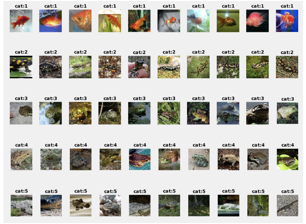
This is a data set with 64x64 sized color images from 200 categories. For HW-2 we only need to deal with 100 images from the first 10 categories, and the following is how to extract the data into ims{} and ids[]:

%%%%%%%%%%%%%%%%%%%%%%%%%%%%%%%

% load Tiny ImageNet data set

%%%%%%%%%%%%%%%%%%%%%%%%%%%%%%%

% get labels

cat_list = dir('~/my.research/dataset/tiny-imagenet-200/train');

n_cat = 10; n_img = 10;

n = 0;

% load images

fork=1:n_cat

ids(k,:) = cat_list(k+2).name;

fprintf(' cat %s', ids(k,:));

flist = dir(sprintf('~/my.research/dataset/tiny-imagenet-200/train/%s/images/*.JPEG',ids(k,:)));

forj=1:n_img

n=n+1; ims{n} = imread(sprintf('~/my.research/dataset/tiny-imagenet-200/train/%s/images/%s',ids(k,:), flist(j+2).name));

fprintf('.');

end

end

% associated labels

ids = kron([1:n_cat], ones(1,n_img))';

% plot

fork=1:n

figure(11);

subplot(5,10,k); imshow(ims{k}); title(sprintf('cat:%d', ids(k)));

end

[1] Use pooled (2x2) color histogram to represent images provide the two following functions for feature extraction and distance computing (codebook can be just fixed 8x4x2 HSV uniform quantization) [20pts]

function [h]=getPooledHSVHistogram(im, codebook, pooling)

function [dist]=getPooledHSVDistance(im1, im2)

[2] Compute HoG feature for image, use the average, as well as 2x2 pooled average as texture feature. Use block size of 8 pixel and 2x2 cell structure. {Hint: use rgb2gray(), vl_hog()} [20pts]

function [hog]=getImHog(im)

function [hog]=getHogDist(h1, h2)

[3] For each image compute its dense SIFT and use Fisher Vector to aggregate. Training SIFT data set for PCA and GMM computation is provided as below, with the training SIFT data at: https://umkc.box.com/s/3shyqe1mkvb6n19arnrusdqstwqms3rs[20pts]

%%%%%%%%%%%%%%%%%%%%%%

% train SIFT PCA, gmm,

%%%%%%%%%%%%%%%%%%%%%%

doTrainGMM=0;

ifdoTrainGMM

% load SIFT training data

load data/hw-2-data.mat;

[A, s, lat]=princomp(double(sift_gmm_km_train));

figure(21); grid on; hold on; plot(lat, '.-');

kd=[16, 24]; nc = [16, 32, 64, 96];

t0=cputime;

forj=1:length(kd)

fork=1:length(nc)

fprintf(' t=%1.2f: GMM: kd(%d)=%d, nc(%d)=%d: ', cputime-t0, j, kd(j), k, nc(k));

% training data reduce dimension via PCA

x = double(sift_gmm_km_train)*A(:,1:kd(j));

% gmm model:

[gmm(j,k).m, gmm(j,k).cov, gmm(j, k).p]=vl_gmm(x', nc(k), 'MaxNumIterations', 30);

end

end

% save PCA and GMM model:

save data/hw2-A-gmm-kd-16-24-nc-16-32-64-96.matAgmm;

else

load data/hw2-A-gmm-kd-16-24-nc-16-32-64-96.matAgmm;

end

create a functions:

function [d]=getSiftFv(sift, A, gmm)

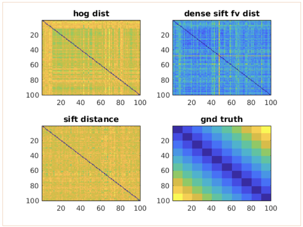
[4] For the 2x2 pooled HSV feature, HoG feature, Fisher Vector aggregated dense SIFT feature, please compute the n x n distance map between all image pairs, and plot their TPR-FPR separately (hint: use vl_roc). 20pts. Examples of distance map:

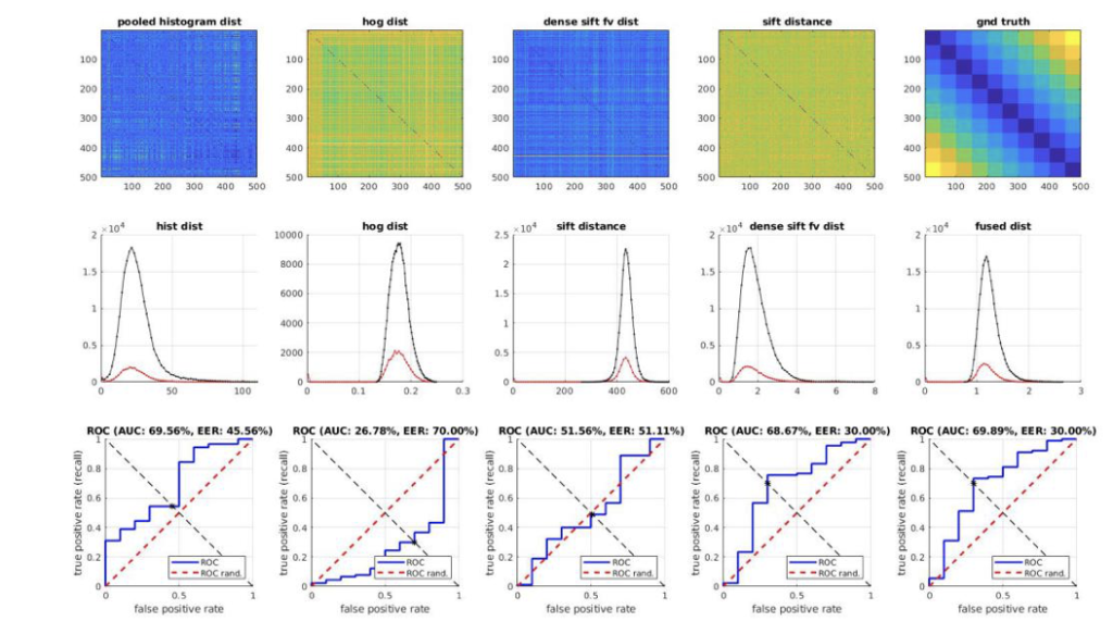
[5] Fuse the distances from different features, and try your own way of finding the best mixing parameters, i.e,

For images and their Color Histogram, HoG, and FV aggregated dense SIFT features respectively. Justify your choice of weights, and plot TPR-FPR ROC curves for different choices. [20pts]

Example: how it should look like:

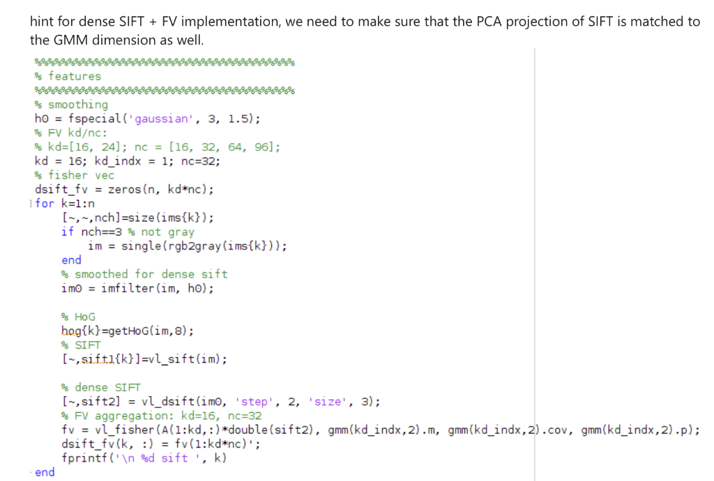
HINT:

hog dist dense sift fv dist 20 40 60 80 100 20 40 60 80 100 20 40 60 80 100 20 40 60 80 100 sift distance gnd truth 20 40 60 80 100 20 40 60 80 100 20 40 60 80 100 20 40 60 80 100 pooled histogram dist hog dist dense sift fy dist sift distance gnd truth 100 200 300 200 200 300 400 500 500 500 500 100 200 300 400 500 100 200 300 400 500 100 200 300 400 500 00 200 300 400 500 100 200 300 400 S00 10 hist dist hog dist 10 sift distance 104 dense sift fv dist x10 fused dist 10000 2.5 1.5 1.5 1.5 1.5 0.5 0.5 0.5 0.1 0.2 0.3 (AUC: 69.56%, EER: 45.56%) ROC (AUC: 26.78%, EER: 70.00%) ROC (AUC: 51.56%, EER: 51.11%) ROC (AUC: 68.67%, EER: 30.00%) ROC (AUC: 69.89%, EER: 30.0 0.8 0.8 0.8 0.8 0.6 0.4 0.8 0.6 0.6 0.6 0.6 0.4 0.4 0.4 0.4 0.2 0.2 0.2 -ROC ROC 0.5 false positive rate 0.5 false positive rate 0.5 false positive rate 0.5 false positive rate 0.5 false positive rate hog dist dense sift fv dist 20 40 60 80 100 20 40 60 80 100 20 40 60 80 100 20 40 60 80 100 sift distance gnd truth 20 40 60 80 100 20 40 60 80 100 20 40 60 80 100 20 40 60 80 100 pooled histogram dist hog dist dense sift fy dist sift distance gnd truth 100 200 300 200 200 300 400 500 500 500 500 100 200 300 400 500 100 200 300 400 500 100 200 300 400 500 00 200 300 400 500 100 200 300 400 S00 10 hist dist hog dist 10 sift distance 104 dense sift fv dist x10 fused dist 10000 2.5 1.5 1.5 1.5 1.5 0.5 0.5 0.5 0.1 0.2 0.3 (AUC: 69.56%, EER: 45.56%) ROC (AUC: 26.78%, EER: 70.00%) ROC (AUC: 51.56%, EER: 51.11%) ROC (AUC: 68.67%, EER: 30.00%) ROC (AUC: 69.89%, EER: 30.0 0.8 0.8 0.8 0.8 0.6 0.4 0.8 0.6 0.6 0.6 0.6 0.4 0.4 0.4 0.4 0.2 0.2 0.2 -ROC ROC 0.5 false positive rate 0.5 false positive rate 0.5 false positive rate 0.5 false positive rate 0.5 false positive rate