please help in answering this question

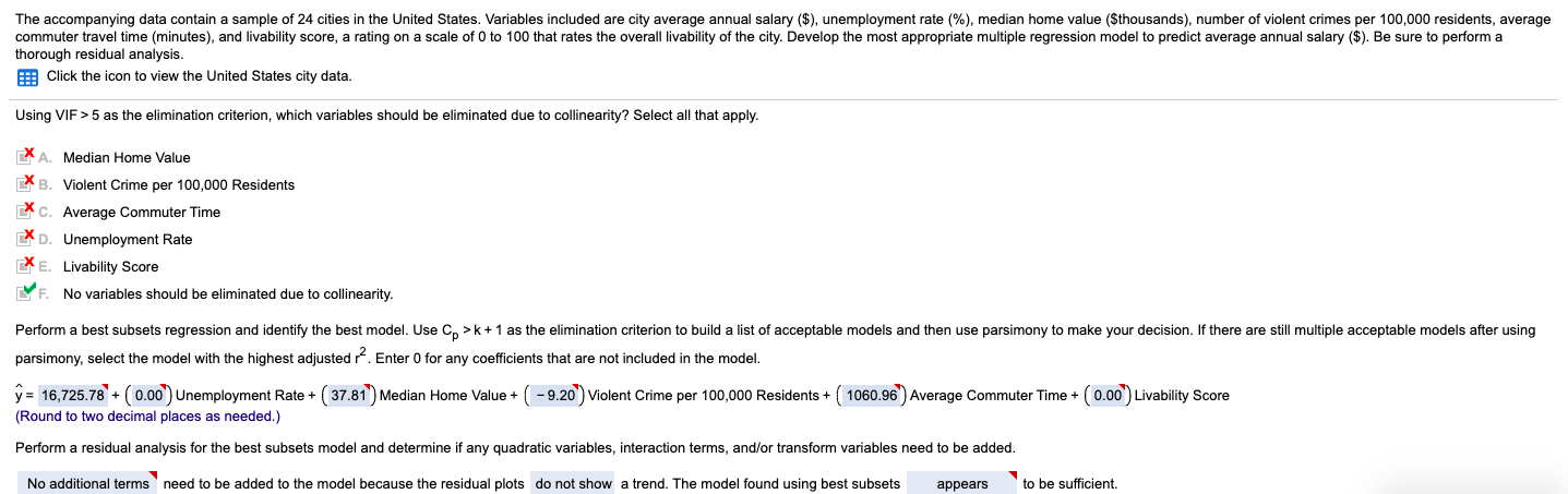
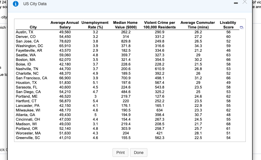
The accompanying data contain a sample of 24 cities in the United States. Variables included are city average annual salary ($), unemployment rate (%), median home value ($thousands), number of violent crimes per 100,000 residents, average commuter travel time (minutes), and livability score, a rating on a scale of 0 to 100 that rates the overall livability of the city. Develop the most appropriate multiple regression model to predict average annual salary ($). Be sure to perform a thorough residual analysis. Click the icon to view the United States city data. Using VIF > 5 as the elimination criterion, which variables should be eliminated due to collinearity? Select all that apply. X A. Median Home Value X B. Violent Crime per 100,000 Residents X C. Average Commuter Time X D. Unemployment Rate X E. Livability Score Y F. No variables should be eliminated due to collinearity. Perform a best subsets regression and identify the best model. Use Co > k + 1 as the elimination criterion to build a list of acceptable models and then use parsimony to make your decision. If there are still multiple acceptable models after using parsimony, select the model with the highest adjusted r. Enter 0 for any coefficients that are not included in the model. y= 16,725.78 + (0.00 ) Unemployment Rate + ( 37.81 ) Median Home Value + ( -9.20 ) Violent Crime per 100,000 Residents + ( 1060.96 ) Average Commuter Time + (0.00 ) Livability Score (Round to two decimal places as needed.) Perform a residual analysis for the best subsets model and determine if any quadratic variables, interaction terms, and/or transform variables need to be added. No additional terms need to be added to the model because the residual plots do not show a trend. The model found using best subsets appears to be sufficient.24 i US City Data of vic / SC e an city Average Annual Unemployment Median Home Violent Crime per Average Commuter Livability lich City Salary Rate (%) Value ($000) 100,000 Residents Time (mins) Score Austin, TX 49,560 3.2 262.2 290.9 26.2 56 Denver, CO 54,450 3.2 314 331.2 27.2 60 San Jose, CA 78,620 3.8 829.8 249.8 26.5 52 Washington, DC 65,910 3.9 371.8 316.6 34.3 59 Fayetteville, AR 43,570 2.9 182.5 334.6 21.2 46 Seattle, WA 59,060 4.8 359.7 327.3 29 63 Boston, MA 62,070 3.5 321.4 354.5 30.2 66 Boise, ID 42,180 3.7 228.6 228.2 21.5 58 Nashville, TN 44,700 3.7 200.6 610.9 26.8 53 le to Charlotte, NC 48,370 4.9 189.5 392.2 26 52 San Francisco, CA 66,900 3.9 700.9 498.1 31.2 66 Houston, TX 51,830 5.1 197.6 567.4 29 49 Sarasota, FL 40,600 4.5 224.6 543.8 23.5 58 San Diego, CA 54,210 4.7 484.6 325.2 25 53 Portland, ME 46,520 3 219.7 127.6 24.6 62 Hartford, CT 56,870 5.4 220 252.2 23.5 58 Lancaster, PA 42,150 4.1 176.1 165.1 22.9 55 Milwaukee, WI 48,170 4.6 190.5 634 23.3 62 Atlanta, GA 49,430 5 194.9 398.4 30.7 48 Cincinnati, OH 47,030 4.4 154.4 267.3 24.5 55 Madison, WI 49,030 3.1 219.4 208.5 21.7 68 Portland, OR 52,140 4.8 303.9 258.7 25.7 61 Worcester, MA 51,630 4.3 204 421 28.1 51 Greenville, SC 41,010 4.6 155.5 562.3 22.5 54 ick d Print Done