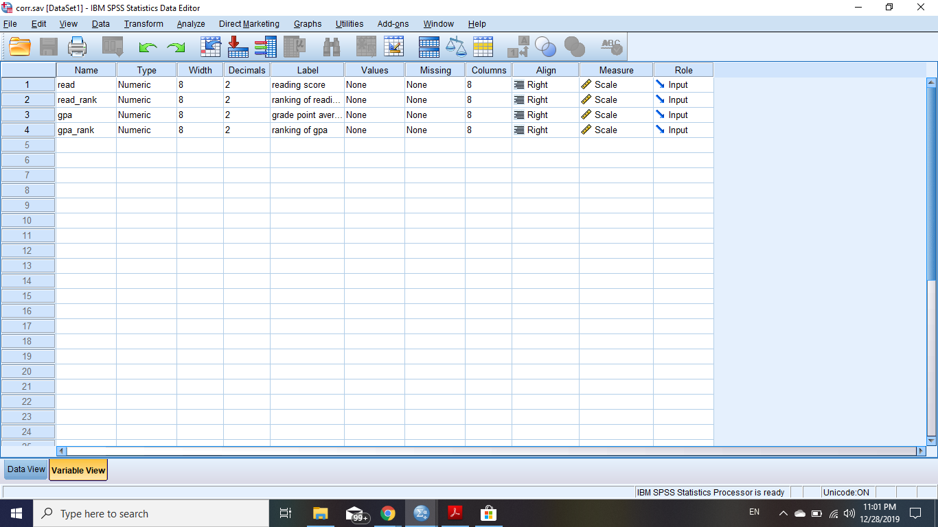
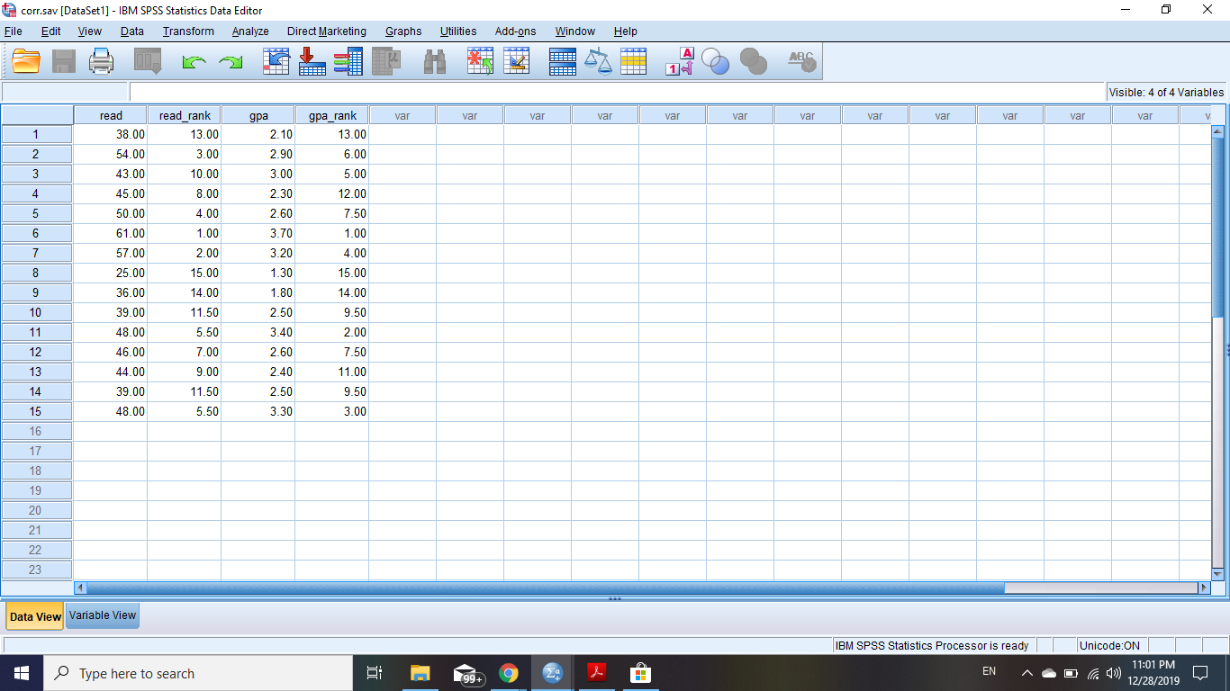
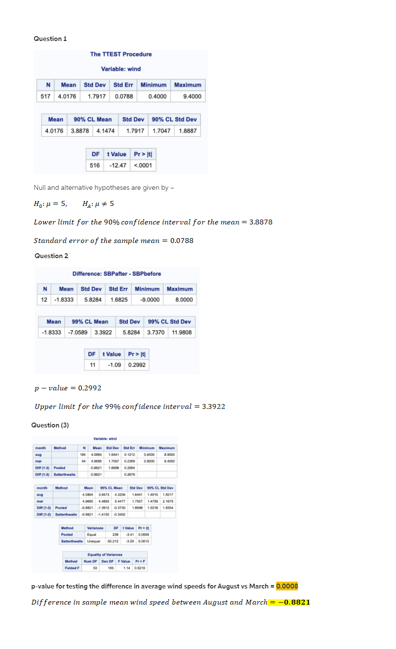
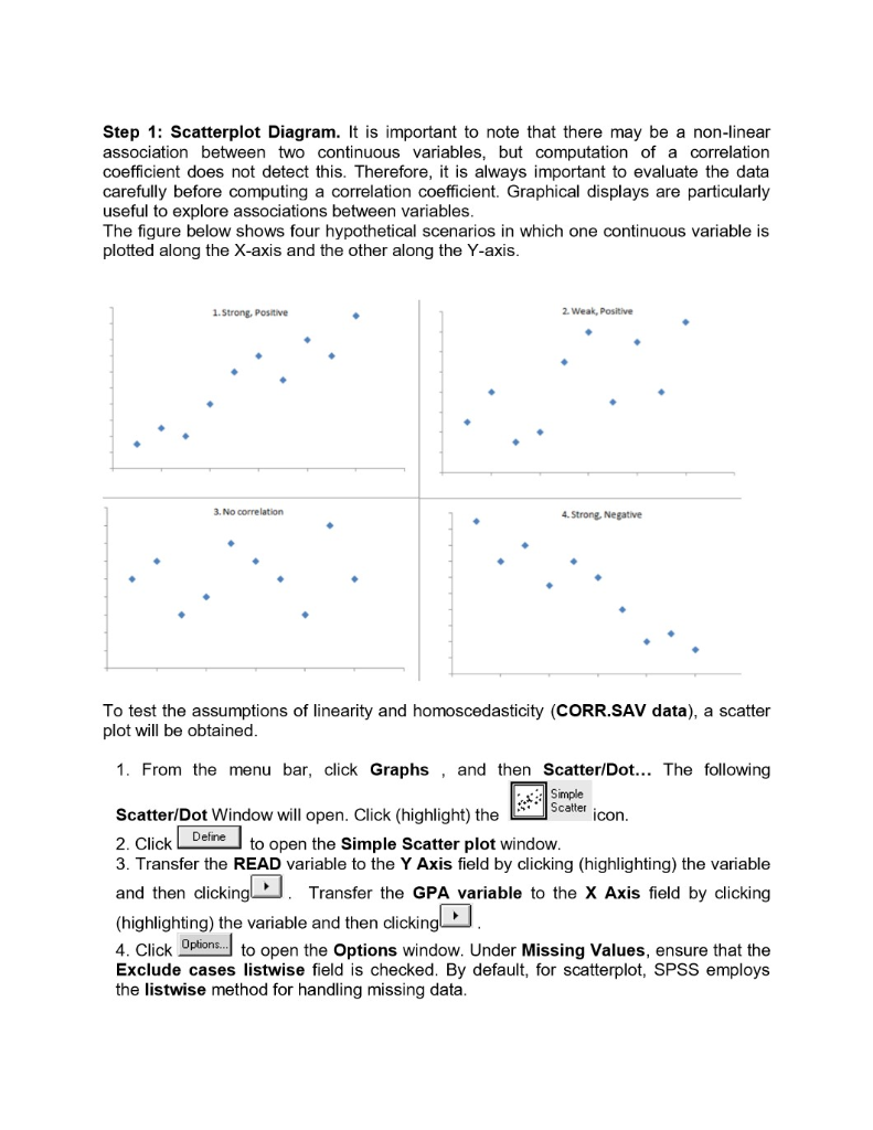
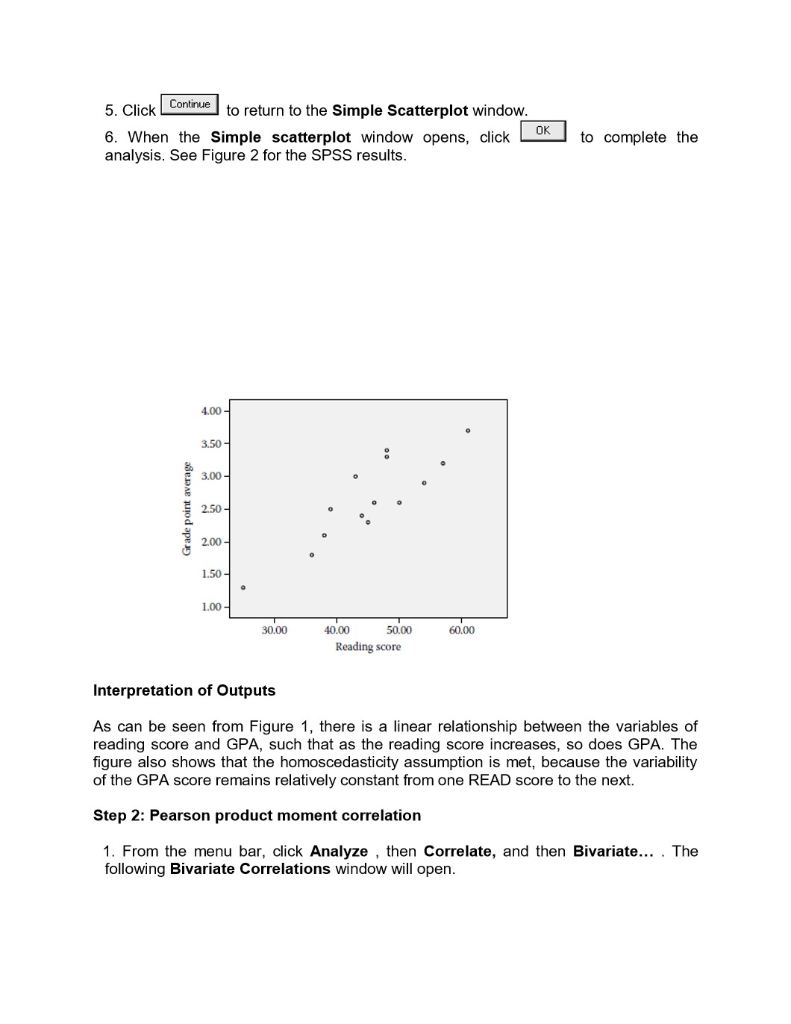
Please help me, I am stump
A major video rental chain recently decided to allow customers to rent movies for three nights rather than one. The marketing team that made the decision reasoned that at least 70% of customers would return the movie by the second night anyway. A sample of 500 customers found 68% returned the movies prior to the third night. A} Given the marketing team's estimate, what would be the probability of a sample result with 68% or fewer returns prior to the third night? Show work 2. The BelSante Company operates retail pharmicies in 10 eastern states. RECENTLY, the company's internal audit department selected selected a randam sample o 300 prescriptions issued throughout the system. The objective of the sampling was to estimate the average dollar value of all prescription issued by the company. the following data was collected : mean = $14.23 and sample standard 3.00. Determine the 90% confidence interval estimate for the true average sales value for prescription issued by the company. Interpret the interval estimate. show work 3. Based on the past experience, the California Power Company forecasts that the mean residential electricity usage per household will be 700 kwh next January. In January the company selects a simple random sample of 49 households and computes a mean of 715. Assume a population standard deviation of 50. Construct a 95% confidence interval for the population mean. Test at the 0.05 level of significance level to determine whether California Power's forecast is reasonable. Compute and interpret the pvalue for the test. Are the results from the confidence interval and the hypothesis testing consistent? Should they be? Justify your answer. corr.sav [DataSet1] - IBM SPSS Statistics Data Editor X File Edit View Data Transform Analyze Direct Marketing Graphs Utilities Add-ons Window Help ABC Name Type Width Decimals Label Values Missing Columns Align Measure Role read Numeric 8 2 reading score None None 8 Right Scale ` Input 2 read rank Numeric 2 ranking of readi... None None CO Right Scale ` Input 3 gpa Numeric 8 2 grade point aver... None None 18 Right Scale \\Input 4 gpa_rank Numeric 8 2 ranking of gpa None None Right Scale \\Input 6 7 8 9 10 11 12 13 14 15 16 17 18 19 20 21 22 23 24 ar Data View| Variable View IBM SPSS Statistics Processor is ready Unicode:ON Type here to search Za EN 11:01 PM 12/28/2019corr.sav [DataSet1] - IBM SPSS Statistics Data Editor X File Edit View Data Transform Analyze Direct Marketing Graphs Utilities Add-ons Window Help A Visible: 4 of 4 Variables read read_rank gpa gpa_rank var var var va var var var var var var var var 38.00 13.00 2.10 13.00 54.00 3.00 2.90 6.00 W N 43.00 10.00 3.00 5.00 45.00 8.00 2.30 12.00 50.00 4.00 2.60 7.50 61.00 1.00 3.70 1.00 57.00 2.00 3.20 4.00 25.00 15.00 1.30 15.00 9 36.00 14.00 1.80 14.00 10 39.00 11.50 2.50 9.50 11 48.00 5.50 3.40 2.00 12 46.00 7.00 2.60 7.50 13 44.00 9.00 2.40 11.00 14 39.00 11.50 2.50 9.50 15 48.00 5.50 3.30 3.00 16 17 18 19 20 21 22 23 1 Data View Variable View IBM SPSS Statistics Processor is ready Unicode:ON + Type here to search EN 11:01 PM 12/28/2019Question 1 The TTEST Procedure Variable: wind N Mean Std Dev Std Err Minimum Maximum 517 4.0176 1.7917 0.0788 0.4000 9.4000 Mean 90% CL Mean Std Dev 90% CL Std Dev 4.0176 3.8878 4.1474 1.7917 1.7047 1.8887 DF t Value Pr > It| 516 -12.47 <.0001 null and alternative hypotheses are given by ho: m="5," ha: h lower limit for the confidence interval mean="3.8878" standard error of sample question difference: sbpafter sbpbefore n std dev err minimum maximum cl df t value pr> It| 11 -1.09 0.2992 p - value = 0.2992 Upper limit for the 99% confidence interval = 3.3922 Question (3) Variable: wind month Method Mean Sid Dev Sid Err Minimum Maximum 10864 1.6441 0.1212 04000 8.9000 mar 1.7557 0.2:389 0.9000 9.4000 Din (1-2) Pooled 0.8821 0 2584 Din (1-2) Safterthwaite -0.8821 0.2679 month Mean 95% CL Mean Bid Dev 95% CL Bid Dev 0864 3.8473 4.3256 1.6441 1.4915 1.8317 4.4893 5.4477 1.7557 1.4759 2.1675 Din (1-2) Pooled 0.8821 -1.3912 -0.3730 1.6898 1.5318 1.8354 Din (1-2) Safterthwaite 0 8821 -1.4150 0.3492 Method Variances DF t Value Pr > FI 236 1 0.0008 Satterthwaite Unequal 82 212 3.29 0.0015 Equality of Variances Method Num OF Den DF F Value Pr >F Folded F 183 1.14 0.5210 p-value for testing the difference in average wind speeds for August vs March = 0.0008 Difference in sample mean wind speed between August and March E -0.8821Correlation Analysis (refer attached photos} please help me with the ff: Survey_perceived stress data The Survey_perceived stress is a set of data from a sample of items: Research Question: Is there significant relationship exist between age and the level of perceived stress? Requirements: a. Using the scatterplot diagram, illustrate the relationship of the two variables. b. Compute the coefficient of correlation. c. How strong is the relationship between Age and Level of Perceived Stress? Explain. another family of regression analysis which is the Logistic regression as well as the Survival analysis. Knowing more about statistics will definitely help in making a scientific decision making as development practitioner in the region. Objectives At the end of the lesson, participants shall be able to: 1. understand the inferential statistical tools particularly correlation and regression analysis; 2. determine which inferential statistical tools appropriate to use based on research questions and gathered data; and 3. use these tools in six-steps hypothesis testing. Discussion/Workshop Module 6: Correlation Analysis Time Allotment: 2 Hours Learning Objectives: At the end of this lesson, you shall be able to: I. test for relationship including magnitude and direction 2. identify and explain types of correlation coefficient 3. describe characteristics common to each of the type 4. recognize assumptions for the test 5. use the software to run data 6. produce SPSS output correlation 7. show and interpret results Overview Correlation is primarily concerned with finding out whether a relationship exists and with determining its magnitude and direction. When two variables vary together, such as loneliness and depression, they are said to be correlated . Accordingly, correlational studies are attempts to find the extent to which two or more variables are related. Typically, in a correlational study, no variables are manipulated as in an experiment the researcher measures naturally occurring events, behaviors, or personality characteristics and then determines if the measured scores covary. The simplest correlational study involves obtaining a pair of observations or measures on two different variables from a number of individuals. The paired measures are then statistically analyzed to determine if any relationship exists between them. For example, behavioral scientists have explored the relationship between variables such as anxiety level and self-esteem, attendance at classes in school and course grades, university performance and career success, and body weight and self-esteem.To quantitatively express the extent to which two variables are related, it is necessary to calculate a correlation coefficient . There are many types of correlation coefficients, and the decision of which one to employ with a specific set of data depends on the following factors: The level of measurement on which each variable is measured . The nature of the underlying distribution (continuous or discrete) . The characteristics of the distribution of the scores (linear or nonlinear) This lesson presents two correlation coefficients: the Pearson product moment correlation coefficient ( r ), employed with interval or ratio scaled variables, and the Spearman rank order correlation coefficient ( r rho ), employed with ordered or ranked data. It is important to note that, regardless of which correlational technique the researcher uses, they all have the following characteristics in common: I. Two sets of measurements are obtained on the same individuals or on pairs of individuals who are matched on some basis. 2. The values of the correlation coefficients vary between +1.00 and -1.00. Both of these extremes represent perfect relationships between the variables, and 0.00 represents the absence of a relationship. 3. A positive relationship means that individuals obtaining high scores on one variable tend to obtain high scores on a second variable. The converse is also true, i.e., individuals scoring low on one variable tend to score low on a second variable. 4. A negative relationship means that individuals scoring low on one variable tend to score high on a second variable. Conversely, individuals scoring high on one variable tend to score low on a second variable. When dealing with population data for two numerical variables, the Greek letter is used as the symbol for the coefficient of correlation. Figure 1 illustrates three different types of association between two variables. . . . . . .. X . X Panel A Panel B Panel C Perfect negative No correlation Perfect positive correlation (p = =1) (p = 0) correlation (p = +1) Correlation alone cannot prove that there is a causation effect-that is, that the change in the value of one variable caused the change in the other variable. A strong correlation can be produced simply by chance, by the effect of a third variable not considered in the calculation of the correlation, or by a cause-and-effect relationship. You would need toperform additional analysis to determine which of these three situations actually produced the correlation. Therefore, you can say that causation implies correlation, but correlation alone does not imply causation. Assumptions 4 For each subject in the study, there must be related pairs of scores, i.e., if a subject has a score on variable X, then the same subject must also have a score on variable Y. The relationship between the two variables must be linear, i.e., the relationship can be most accurately represented by a straight line. + The variables should be measured at least at the interval level. The variability of scores on the Y variable should remain constant at all values of the X variable. This assumption is called homoscedasticity. Hands-on Activity Assume that a researcher wishes to determine whether there is a relationship between grade point average (GPA) and the scores on a reading-comprehension test of 15 first- year students. The researcher recorded the pair of scores given in the following, together with their rankings: Correlation Student Read Read_rank GPA GPA_rank S 38 13 2. 1 $2 54 2.9 $3 43 10 3.0 45 2.3 12 $5 50 4 2.6 7.5 56 61 I 3.7 $7 57 N 3.2 SPSS Data Needed: $8 25 15 1.3 15 $9 36 14 1.8 14 The data set has been saved under the name: CORR.SAV $10 39 1 1.5 2.5 9.5 Variable Column(s) Code sll 5.5 3.4 2 46 2.6 7.5 READ $ 1 3 44 Reading score 11 READ_RANK Ranking 1 1.3 25 9.5 Steps in SPSS $15 5.5 3.3 wStep 1: Scatterplot Diagram. It is important to note that there may be a non-linear association between two continuous variables, but computation of a correlation coefficient does not detect this. Therefore, it is always important to evaluate the data carefully before computing a correlation coefficient. Graphical displays are particularly useful to explore associations between variables. The figure below shows four hypothetical scenarios in which one continuous variable is plotted along the X-axis and the other along the Y-axis. 1. Strong, Positive 2. Weak, Positive 3. No correlation 4. Strong, Negative To test the assumptions of linearity and homoscedasticity (CORR.SAV data), a scatter plot will be obtained. 1. From the menu bar, click Graphs , and then Scatter/Dot... The following Simple Scatter/Dot Window will open. Click (highlight) the Scatter icon. 2. Click Define to open the Simple Scatter plot window. 3. Transfer the READ variable to the Y Axis field by clicking (highlighting) the variable and then clicking' . Transfer the GPA variable to the X Axis field by clicking (highlighting) the variable and then clicking 4. Click Options.] to open the Options window. Under Missing Values, ensure that the Exclude cases listwise field is checked. By default, for scatterplot, SPSS employs the listwise method for handling missing data.5. Click Continue to return to the Simple Scatterplot window. 6. When the Simple scatterplot window opens, click OK to complete the analysis. See Figure 2 for the SPSS results. 4.00- 3.50- 3.00 - Grade point average 2.50- 2.00 - 1.50- 1.00 30.00 40.00 50.00 60.00 Reading score Interpretation of Outputs As can be seen from Figure 1, there is a linear relationship between the variables of reading score and GPA, such that as the reading score increases, so does GPA. The figure also shows that the homoscedasticity assumption is met, because the variability of the GPA score remains relatively constant from one READ score to the next. Step 2: Pearson product moment correlation 1. From the menu bar, click Analyze , then Correlate, and then Bivariate... . The following Bivariate Correlations window will open.2. Transfer the READ and GPA variables to the Variables field by clicking (highlighting) them and then clicking . By default, SPSS will employ the Pearson correlation analysis, and a two-tailed test of significance (both fields are checked). 3. Click Options.] to open the Bivariate Correlation: Options window. By default, SPSS employs the Exclude cases pairwise method for handling missing data (this field is checked). This method treats the calculation of each pair of variables as a separate problem, using all cases with complete data for the pair. With this method, only cases with missing data on a specific pair of variables will be excluded from the calculation. As such, the correlation for different pairs of variables may be based on different number of cases. As an option, the Exclude cases listwise method can be used to include only those cases with complete data. With this method, any case with missing data on any pair of variables will be excluded from the calculation. As such, the sample size for the correlation between any pair of variables can be reduced further with the listwise method. 4. Click Continue to return to the Bivariate Correlations window. 5. When the Bivariate Correlations window opens, click OK to complete the analysis. See Table 10.1 for the results. Results and Interpretation The correlation between reading score and GPA is positive and statistically significant (r = 0.867, p