

Answered step by step
Verified Expert Solution
Question
1 Approved Answer
please help me step by step i am struggling alot thank you so much! Project Description: In the following project, you will create a worksheet
please help me step by step i am struggling alot
Project Description: In the following project, you will create a worksheet comparing the sales of different types of oven steamers sold in the second quarter. Steps to Perform: 7573,3.85 for January and 68541.64 for February and 82955,31 for March. Max users: Widen column A to 21.83 (136 pixels) and colamns B.F to 13.83 (88 pixels). 6 In cell B8, on the Home tab, ase the AutoSum batton to sum the January sales. 10 Copy the fesulting formula across to cells C8:Ds to sam the February monthly sales and the Manch monthly sales. In cell E4, use the AutoSum batton to sur the Chef Master Steamer sales. Copy the formula down to cells E5:F8. 7 Apply the Heading 4 cell style to the row tisles and columin titles, and then apply 6 the Total cell style to the totals in the range BS:E8. 8 Apply the Accounting Number Format to the first row of sales figures and to the 6 total row, Apply the Comma Style to the remaining sales figures. 9. To compare the monthly sales of each product visually, select the range that 10 represents the sales figures for the three months, including the moeth names and the product names - do not include any lotals in the range. With this data selketed, use the Resoenmended Charts command to insert a Clustered Column chart with the month namses displayed on the category axis and the product names displayed in the legend. 10 Move the chart so that its apper left eorner is positioned in the eenter of cell 3 Alo. Then drag the center right siring handle to the night until the right edge of the chant aligns with the right edge of column E; this will display the legend on one row and, after you add the sparklines, center the chart below the data. 11 Apply Chart Style 5 and change the colors by applying the third tow of colors 13 under Colorful. Change the Chat Title to First Quarter Ovea Steamer Sales 12 In the range F4:F7, insert Line sparklines that compare the monthly data. Do not 10 include the totals. Show the sparkline Markers. Display the sparkline Style gallery, and then is the second row, apply the firs style. 13 Center the workshoet Horizontally on the page, and then insert a Fooker with the 6 File Name in the left section. 14 Change the Orientation to Landscape. Display the document properties, and then 6 as the Tags type steamer sales As the Subject, type your course nume and section number. Be sure your narse displays as the Auther. Check your worksheet by previewing it in Print Preview, and then make any nccessary corrections. 15 Save and close the workbook, and then submit for grading. 0 Total Points 100 thank you so much! 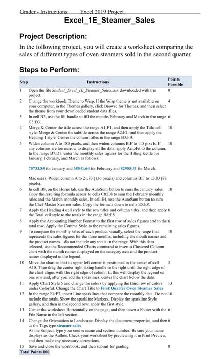
Step by Step Solution
There are 3 Steps involved in it
Step: 1

Get Instant Access to Expert-Tailored Solutions
See step-by-step solutions with expert insights and AI powered tools for academic success
Step: 2

Step: 3
Ace Your Homework with AI
Get the answers you need in no time with our AI-driven, step-by-step assistance
Get Started
Information For Decision Making Readings In Cost And Managerial Accounting
Authors: Alfred Rappaport
3rd Edition
0134643542, 978-0134643540