Please help me to answer this question?

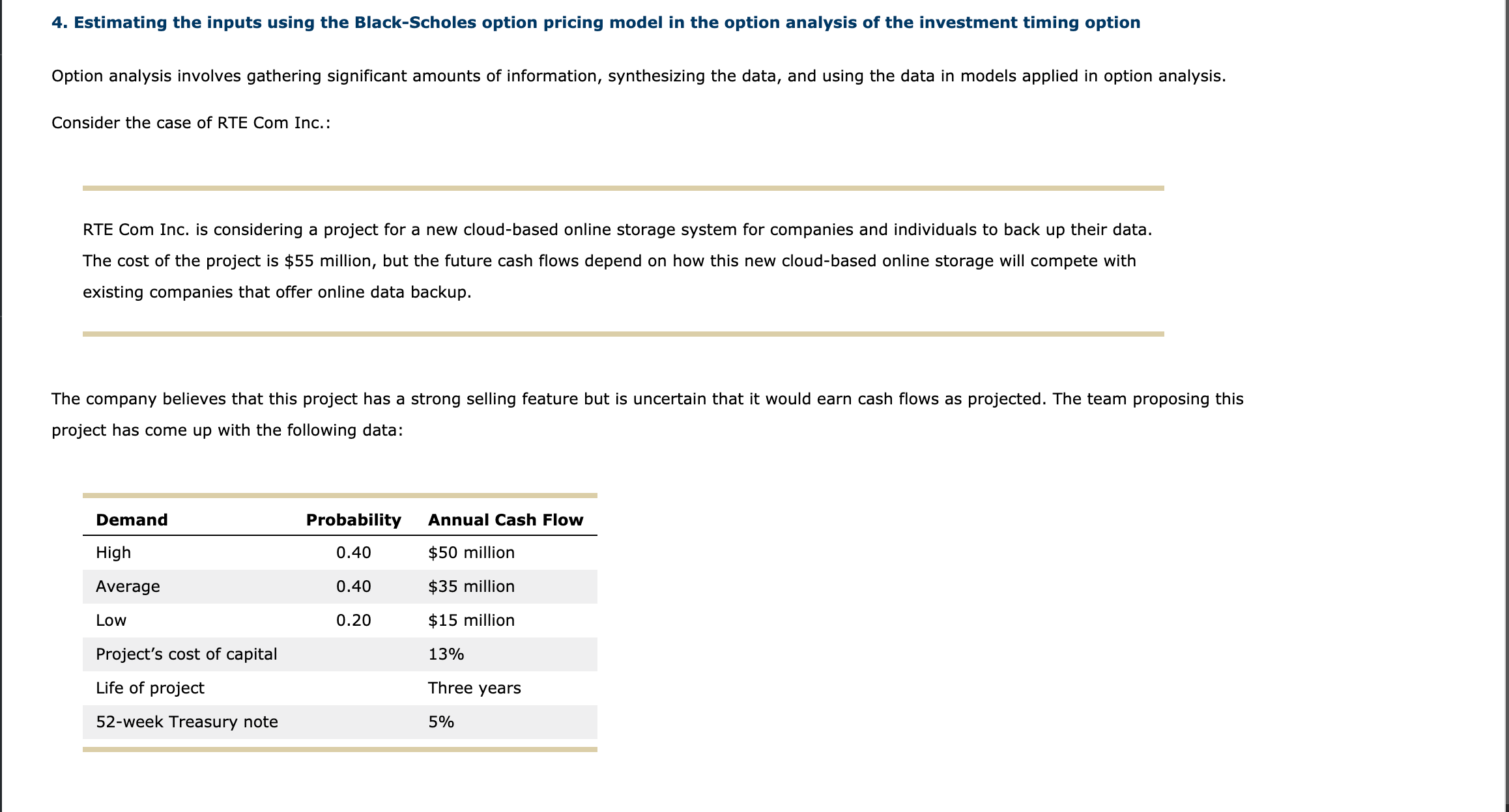
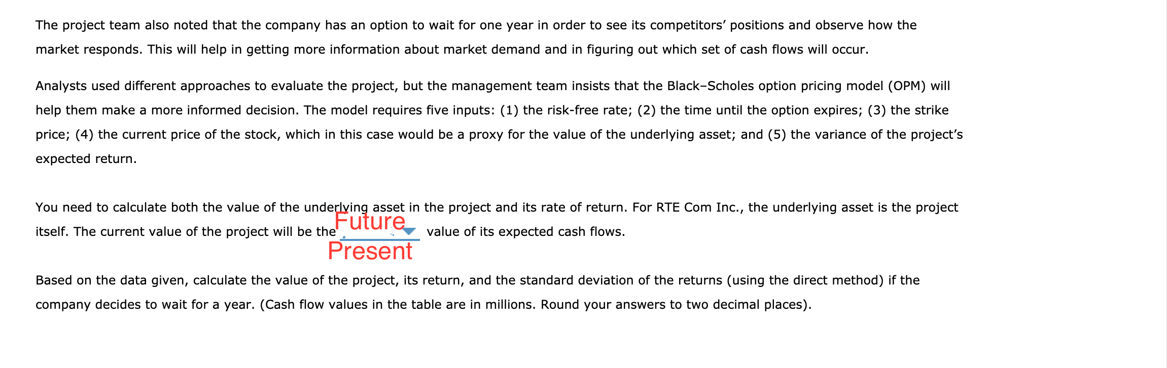
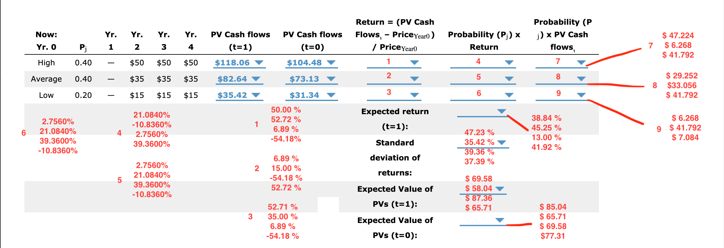
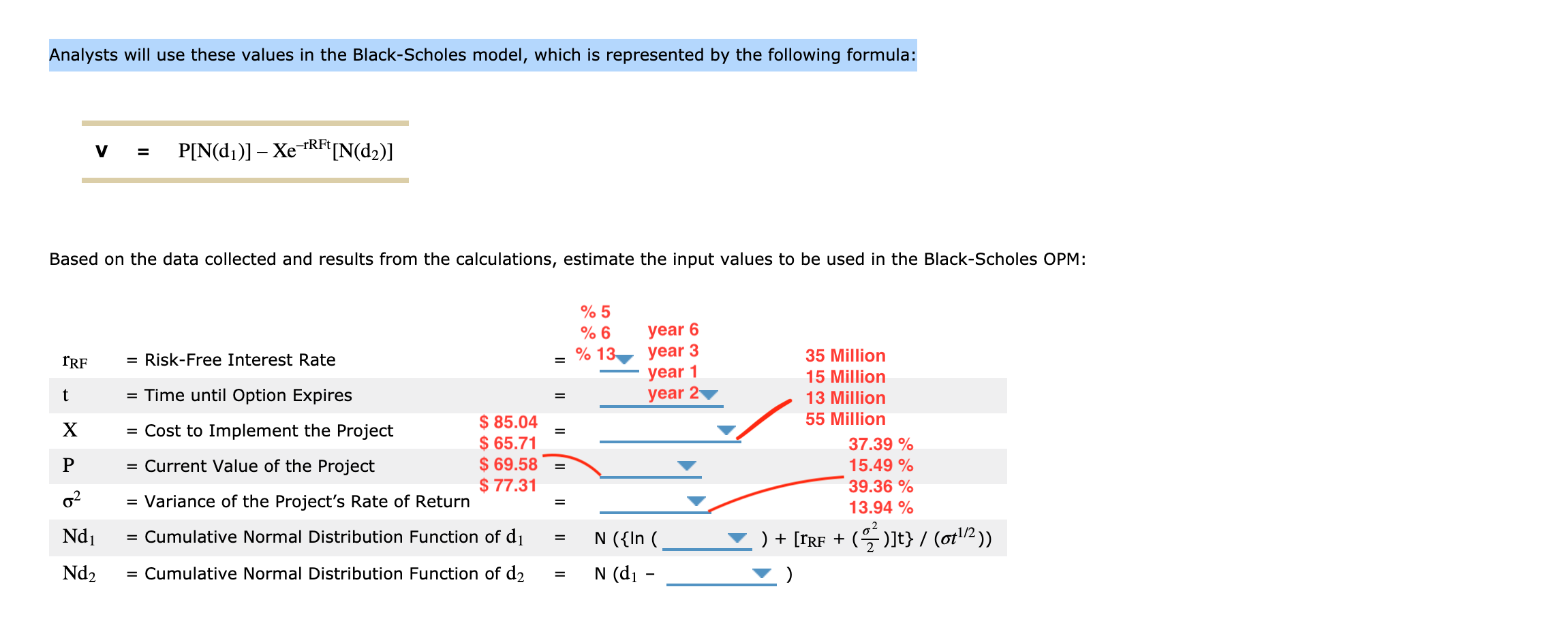
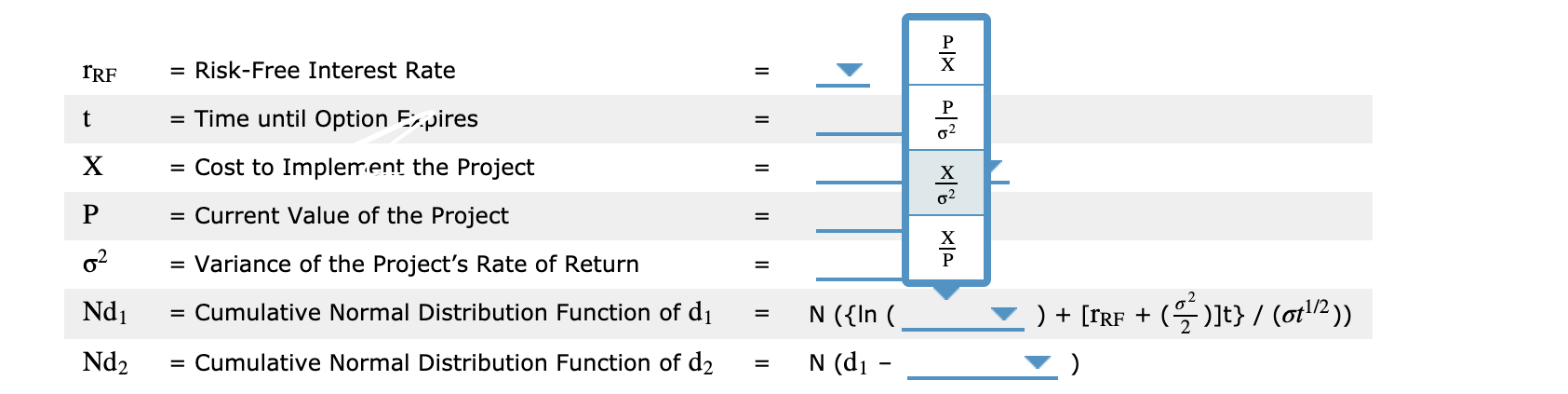
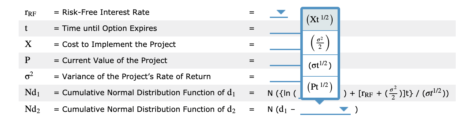
4. Estimating the inputs using the BIack-Scholes option pricing model in the option analysis of the investment timing option Option analysis involves gathering signicant amounts of information, synthesizing the data, and using the data in models applied in option analysis. Consider the case of RTE Com Inc.: RTE Com Inc. is considering a project for a new cloud-based online storage system for companies and individuals to back up their data. The cost of the project is $55 million, but the future cash flows depend on how this new cloud-based online storage will compete with existing companies that offer online data backup. The company believes that this project has a strong selling feature but is uncertain that it would earn cash flows as projected. The team proposing this project has come up with the following data: Demand Probability Annual Cash Flow High 0.40 $50 million Average 0.40 $35 million Low 0.20 $15 million Project's cost of capital 13% Life of project Three years 52-week Treasury note 5% The project team also noted that the company has an option to wait for one year in order to see its competitors' positions and observe how the market responds. This will help in getting more information about market demand and in guring out which set of cash ows will occur. Analysts used different approaches to evaluate the project, but the management team insists that the BlackScholes option pricing model (0PM) will help them make a more informed decision. The model requires five inputs: (1) the risk-free rate; (2) the time until the option expires; (3) the strike price; (4) the current price of the stock, which in this case would be a proxy for the value of the underlying asset; and (5) the variance of the project's expected return. You need to calculate both the value of the undeijgin asset in the project and its rate of return. For RTE Com Inc., the underlying asset is the project itself. The current value of the project will be the _ U \"Kev value of its expected cash flows. Present Based on the data given, calculate the value of the project, its return, and the standard deviation of the returns (using the direct method) if the company decides to wait for a year. (Cash flow values in the table are in millions. Round your answers to two decimal places). Return = (PV Cash Probability (P Now: Yr. Yr. Yr. Yr. PV Cash flows PV Cash flows Flows, - PriceYear0 ) Probability (P;) x j) x PV Cash $ 47.224 Yr. 0 Pi 1 2 3 4 (t=1) (t=0) / PriceYear0 Return flows 7 $ 6.268 $ 41.792 High 0.40 $50 $50 $50 $118.06 $104.48 4 7 Average 0.40 $35 $35 $35 $82.64 $73.13 2 5 8 $ 29.252 8 $33.056 Low 0.20 $15 $15 $15 $35.42 $31.34 3 6 9 $ 41.792 21.0840% 50.00 % Expected return 52.72 % 38.84 % $ 6.268 2.7560% -10.8360% 1 21.0840% 6.89 % (t=1): $ 41.792 6 4 2.7560% 47.23 % 45.25 % 9 39.3600% -54.18% 13.00 % $ 7.084 39.3600% Standard 35.42 % 39.36 % 41.92 % -10.8360% 6.89 % deviation of 2.7560% 37.39 % 2 15.00 % 21.0840% returns: 5 -54.18 % $ 69.58 39.3600% 52.72 % Expected Value of $ 58.04 -10.8360% $ 87.36 52.71 % PVs (t=1): $ 65.71 $ 85.04 3 35.00 % Expected Value of $ 65.71 6.89% $ 69.58 -54.18 % PVs (t=0): $77.31Analysts will use these values in the Black-Scholes model, which is represented by the following formula: V = P[N(d1)] - Xe TRFi [N(d2)] Based on the data collected and results from the calculations, estimate the input values to be used in the Black-Scholes OPM: % 5 % 6 year 6 = Risk-Free Interest Rate = % 13 year 3 IRF 35 Million year 1 15 Million t = Time until Option Expires year 2 13 Million X = Cost to Implement the Project $ 85.04 55 Million = $ 65.71 37.39 % P = Current Value of the Project $ 69.58 = 15.49 % $ 77.31 39.36 % 02 = Variance of the Project's Rate of Return 13.94 % Nd1 = Cumulative Normal Distribution Function of dj = N ({In ( ) + [ IRF + (" ) ]t} / (0+1/2) ) Nd2 = Cumulative Normal Distribution Function of d2 = N (d1 -1 aawwa 2 = Risk-Free Interest Rate = Time until Option Expires = Cost to Implement the Project = Current Value of the Project = Variance of the Project's Rate of Return = Cumulative Normal Distribution Function of (11 = Cumulative Normal Distribution Function of d; aawwa = RiskFree Interest Rate = Time until Option Expires = Cost to Implement the Project = Current Value of the Project = Variance of the Project's Rate of Return = Cumulative Normal Distribution Function of (11 ) + [mm + (072)]t} / (0115)) ll 2 9- I 4 V = Cumulative Normal Distribution Function of d2