 PLEASE HELP ME WITH Q2C. THANK YOU
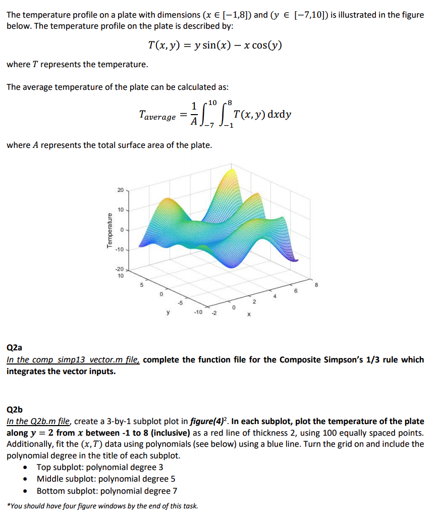
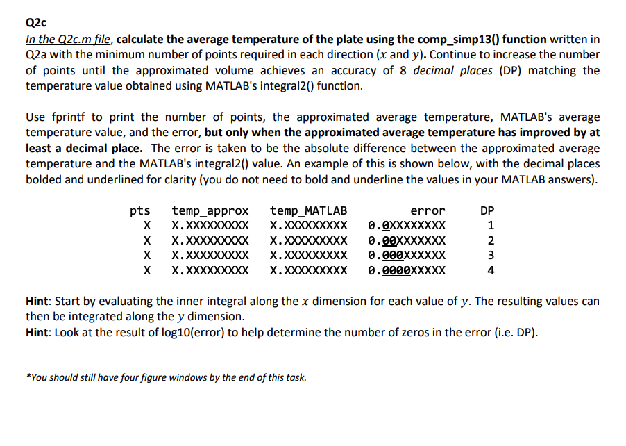
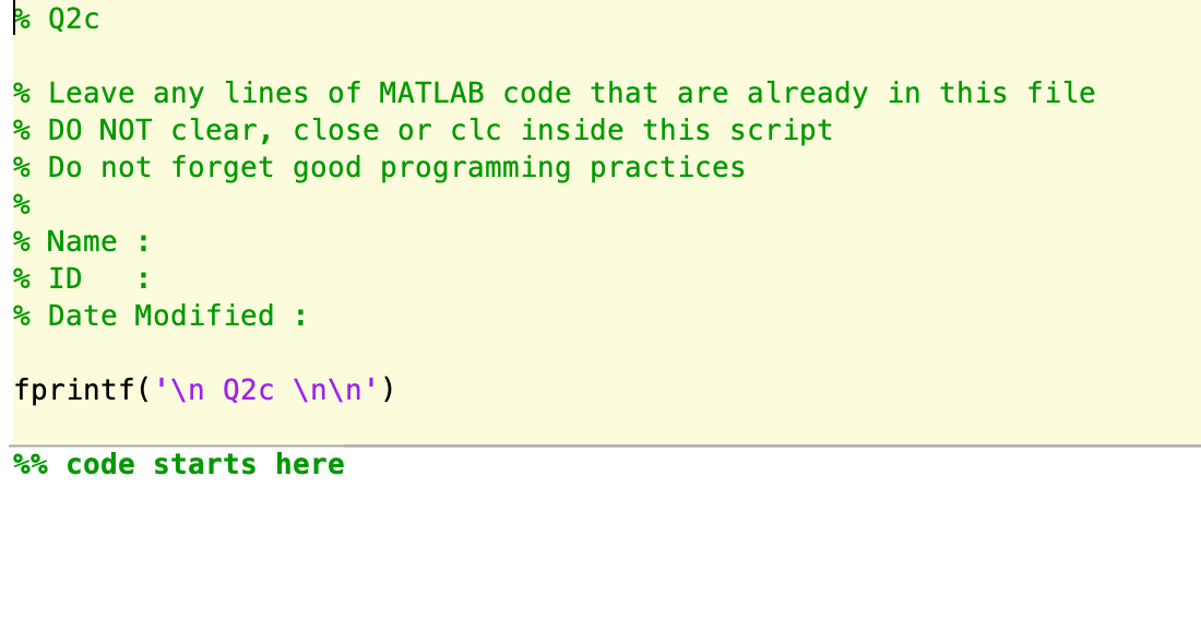
The temperature profile on a plate with dimensions (x E [-1,8]) and (y e [-7,10]) is illustrated in the figure below. The temperature profile on the plate is described by: T(x, y) = y sin(x) x cos(y) where T represents the temperature. The average temperature of the plate can be calculated as: 8" T(, ) dxdy 10 Taverage where A represents the total surface area of the plate. 20 10 - -10 - -20 10 -5 -10 -2 Q2a In the comp simp13 vector.m file, complete the function file for the Composite Simpson's 1/3 rule which integrates the vector inputs. Q2b In the Q2b.m file, create a 3-by-1 subplot plot in figure(4). In each subplot, plot the temperature of the plate along y = 2 from x between -1 to 8 (inclusive) as a red line of thickness 2, using 100 equally spaced points. Additionally, fit the (x,T) data using polynomials (see below) using a blue line. Turn the grid on and include the polynomial degree in the title of each subplot. Top subplot: polynomial degree 3 Middle subplot: polynomial degree 5 Bottom subplot: polynomial degree 7 *You should have four figure windows by the end of this task. Temperature Q2c In the Q2c.m file, calculate the average temperature of the plate using the comp_simp13() function written in Q2a with the minimum number of points required in each direction (x and y). Continue to increase the number of points until the approximated volume achieves an accuracy of 8 decimal places (DP) matching the temperature value obtained using MATLAB's integral2() function. Use fprintf to print the number of points, the approximated average temperature, MATLAB'S average temperature value, and the error, but only when the approximated average temperature has improved by at least a decimal place. The error is taken to be the absolute difference between the approximated average temperature and the MATLAB's integral2() value. An example of this is shown below, with the decimal places bolded and underlined for clarity (you do not need to bold and underline the values in your MATLAB answers). DP temp_MATLAB pts temp_approx error X.XXXXXXXXX .XXXXXXXX 0.0XXXXXXXX 0.00XXXXXXX 0.00XXXXX 0.0000XXXXX X.XXXXXXXXX .XXXXXXXX X.XXXXXXXXX X.XXXXXXXXX 3 . XXXXXXXXX .XXXXXXXX 4 Hint: Start by evaluating the inner integral along the x dimension for each value of y. The resulting values can then be integrated along the y dimension. Hint: Look at the result of log10(error) to help determine the number of zeros in the error (i.e. DP). *You should still have four figure windows by the end of this task. P% Q2c % Leave any lines of MATLAB code that are already in this file % DO NOT clear, close or clc inside this script % Do not forget good programming practices % Name : % ID % Date Modified : fprintf(' Q2c ') %% code starts here The temperature profile on a plate with dimensions (x E [-1,8]) and (y e [-7,10]) is illustrated in the figure below. The temperature profile on the plate is described by: T(x, y) = y sin(x) x cos(y) where T represents the temperature. The average temperature of the plate can be calculated as: 8" T(, ) dxdy 10 Taverage where A represents the total surface area of the plate. 20 10 - -10 - -20 10 -5 -10 -2 Q2a In the comp simp13 vector.m file, complete the function file for the Composite Simpson's 1/3 rule which integrates the vector inputs. Q2b In the Q2b.m file, create a 3-by-1 subplot plot in figure(4). In each subplot, plot the temperature of the plate along y = 2 from x between -1 to 8 (inclusive) as a red line of thickness 2, using 100 equally spaced points. Additionally, fit the (x,T) data using polynomials (see below) using a blue line. Turn the grid on and include the polynomial degree in the title of each subplot. Top subplot: polynomial degree 3 Middle subplot: polynomial degree 5 Bottom subplot: polynomial degree 7 *You should have four figure windows by the end of this task. Temperature Q2c In the Q2c.m file, calculate the average temperature of the plate using the comp_simp13() function written in Q2a with the minimum number of points required in each direction (x and y). Continue to increase the number of points until the approximated volume achieves an accuracy of 8 decimal places (DP) matching the temperature value obtained using MATLAB's integral2() function. Use fprintf to print the number of points, the approximated average temperature, MATLAB'S average temperature value, and the error, but only when the approximated average temperature has improved by at least a decimal place. The error is taken to be the absolute difference between the approximated average temperature and the MATLAB's integral2() value. An example of this is shown below, with the decimal places bolded and underlined for clarity (you do not need to bold and underline the values in your MATLAB answers). DP temp_MATLAB pts temp_approx error X.XXXXXXXXX .XXXXXXXX 0.0XXXXXXXX 0.00XXXXXXX 0.00XXXXX 0.0000XXXXX X.XXXXXXXXX .XXXXXXXX X.XXXXXXXXX X.XXXXXXXXX 3 . XXXXXXXXX .XXXXXXXX 4 Hint: Start by evaluating the inner integral along the x dimension for each value of y. The resulting values can then be integrated along the y dimension. Hint: Look at the result of log10(error) to help determine the number of zeros in the error (i.e. DP). *You should still have four figure windows by the end of this task. P% Q2c % Leave any lines of MATLAB code that are already in this file % DO NOT clear, close or clc inside this script % Do not forget good programming practices % Name : % ID % Date Modified : fprintf(' Q2c ') %% code starts here


 PLEASE HELP ME WITH Q2C. THANK YOU


