

Question: Please help me with whatever you can with this assignment f9.1 The Motivation for an Analysis of Variance 355 You will notice that this sampling
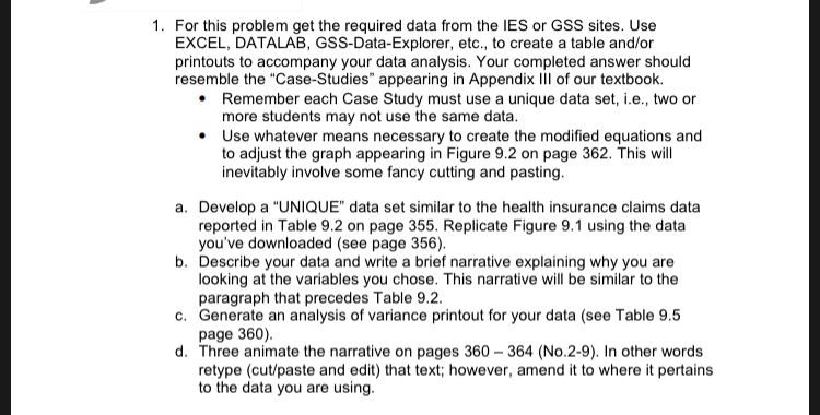
Please help me with whatever you can with this assignment
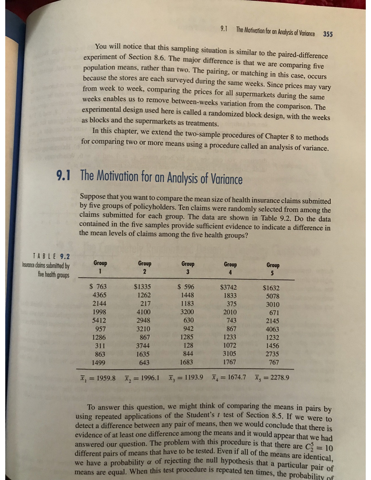
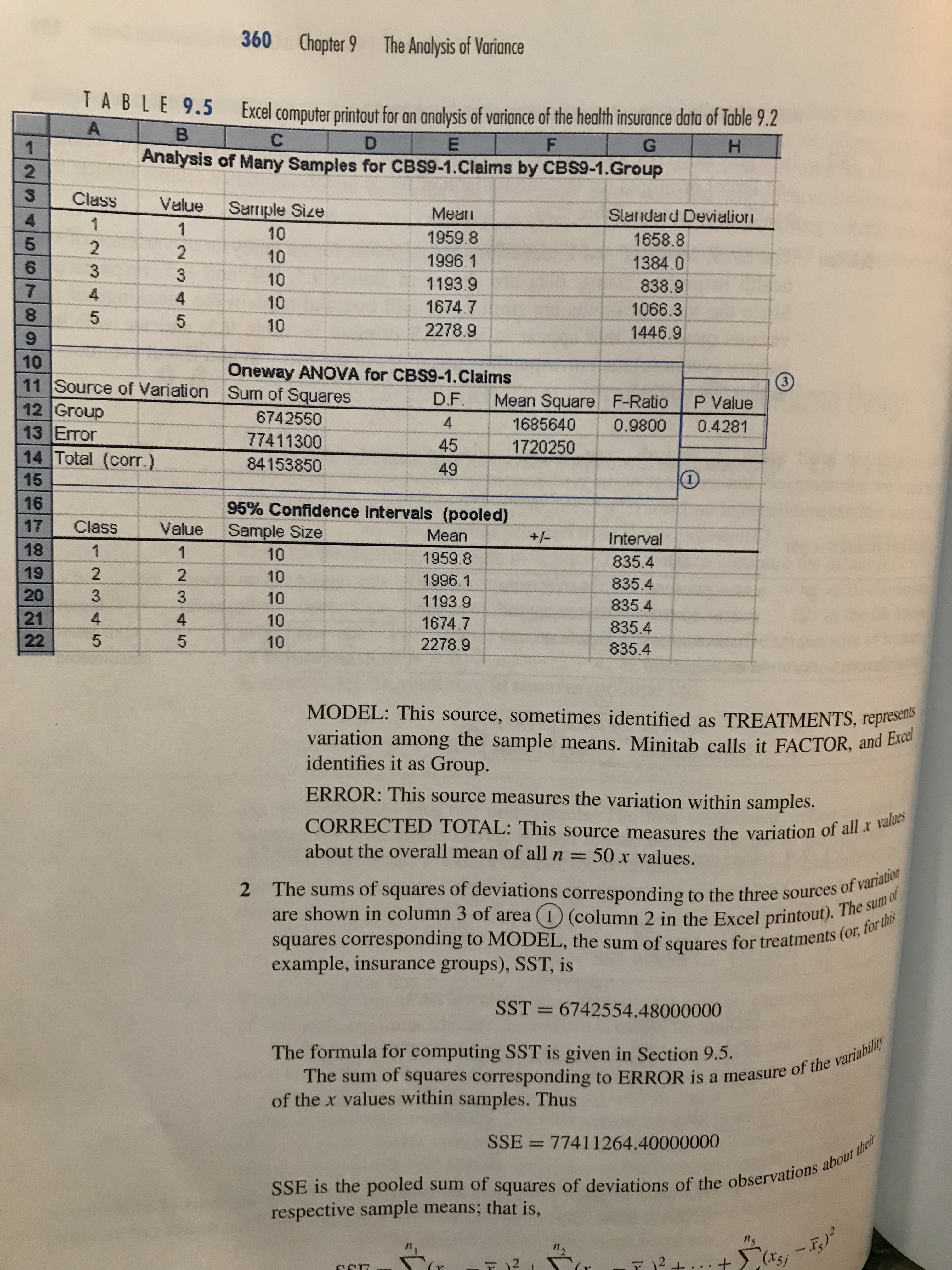
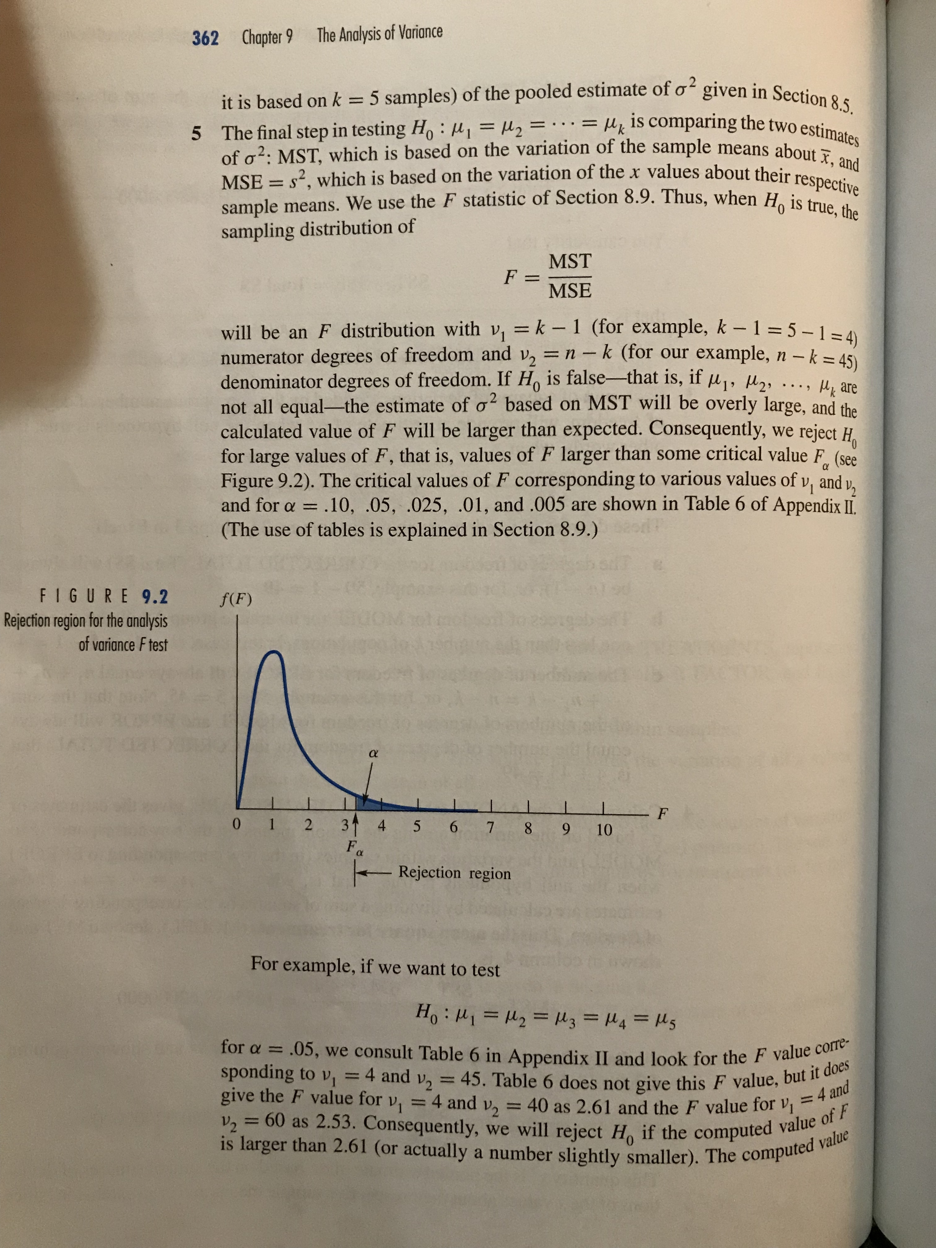
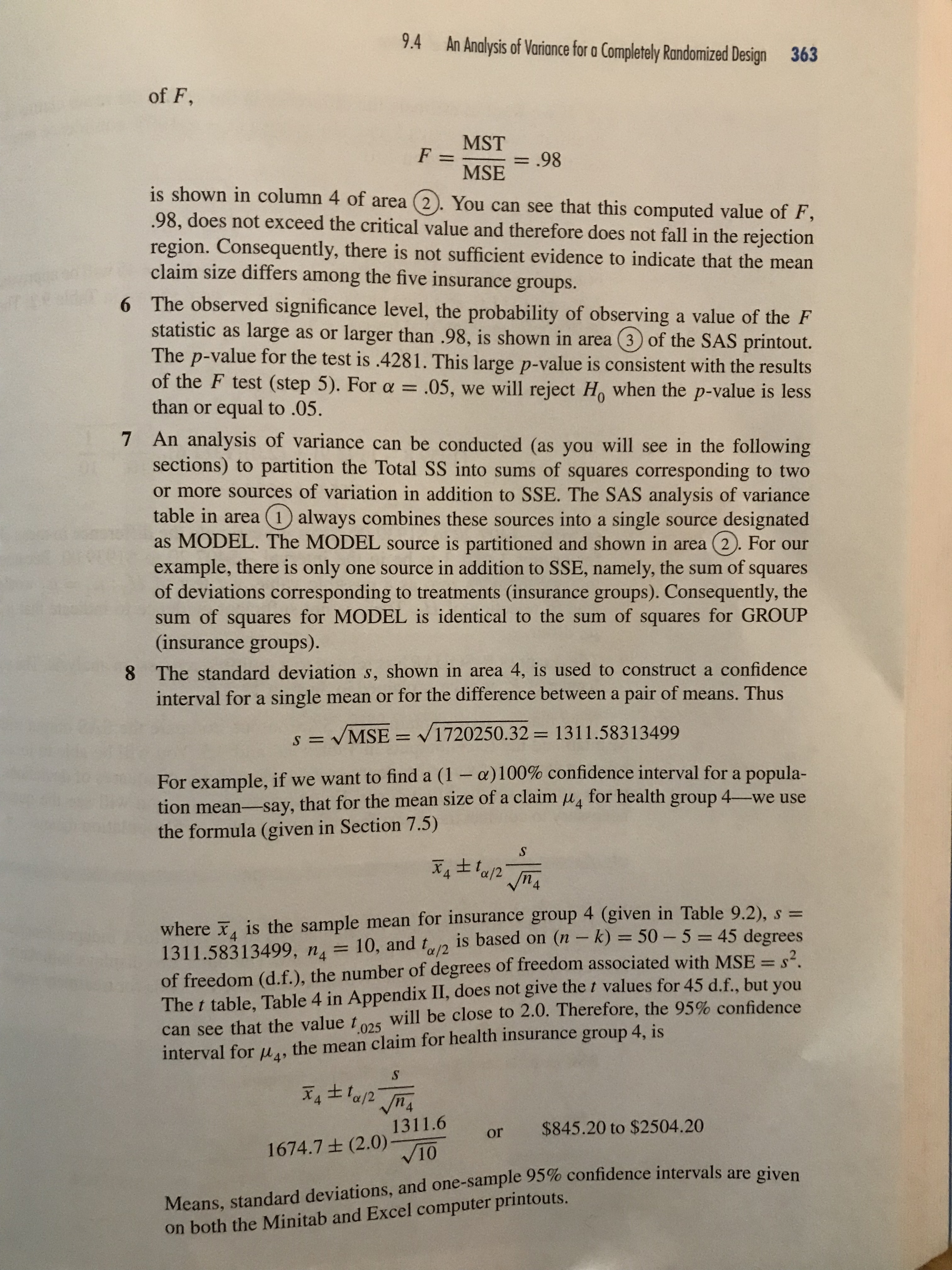
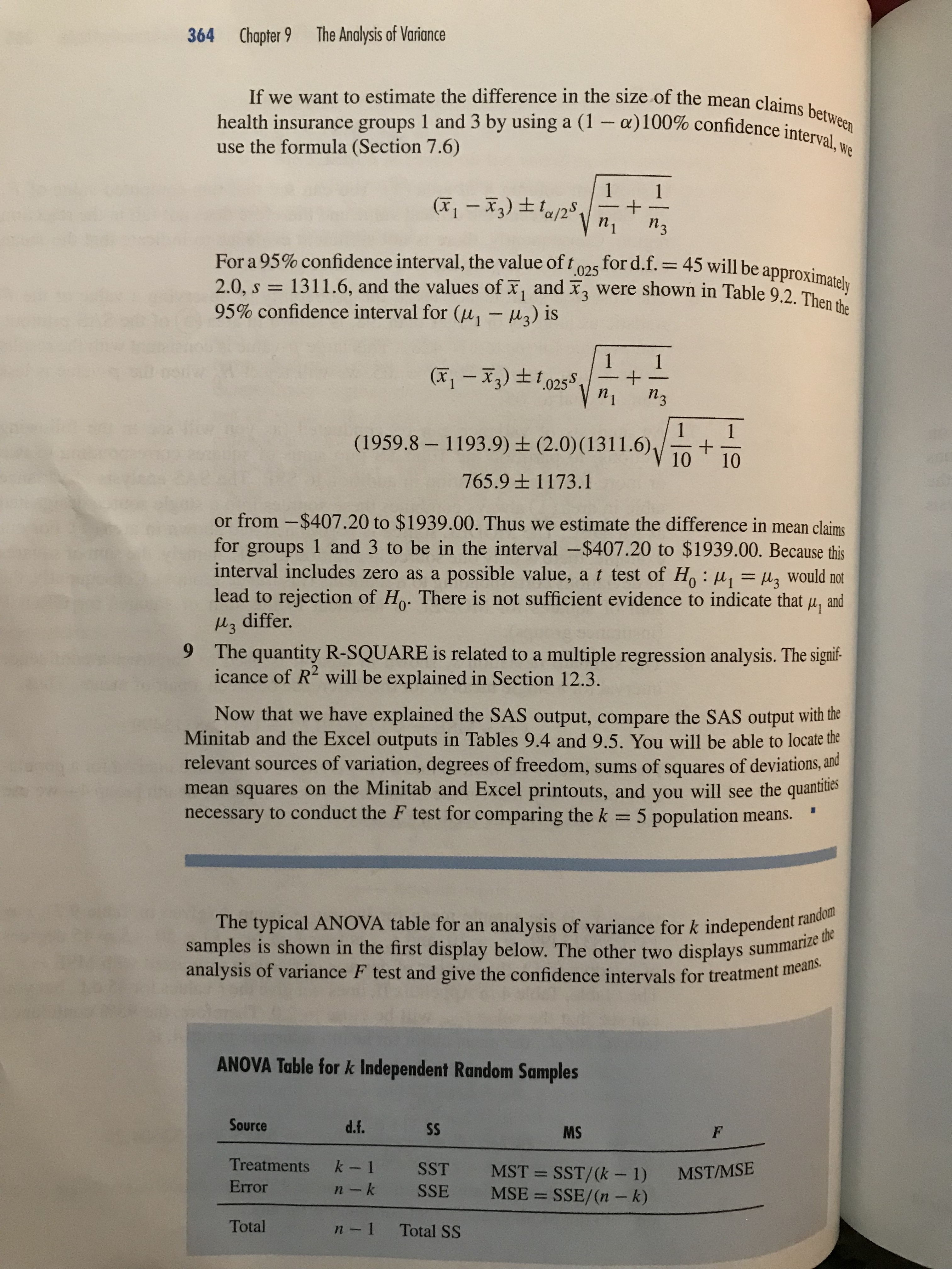
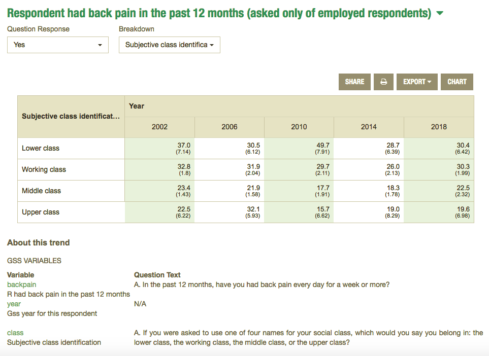
\f9.1 The Motivation for an Analysis of Variance 355 You will notice that this sampling situation is similar to the paired - difference experiment of Section 8. 6 . The major difference is that we are comparing five population means , rather than two . The pairing , or matching in this case , occurs because the stores are each surveyed during the same weeks . Since prices may vary from week to week , comparing the prices for all supermarkets during the same weeks enables us to remove between - weeks variation from the comparison . The experimental design used here is called a randomized block design , with the weeks as blocks and the supermarkets as treatments . In this chapter , we extend the two - sample procedures of Chapter & to methods for comparing two or more means using a procedure called an analysis of variance . 9 . 1 The Motivation for an Analysis of Variance Suppose that you want to compare the mean size of health insurance claims submitted by five groups of policyholders . Ten claims were randomly selected from among the claims submitted for each group . The data are shown in Table 9 .2 . Do the data contained in the five samples provide sufficient evidence to indicate a difference in the mean levels of claims among the five health groups ?! TABLE 9 . 2 surance claims submitted by Group Group Group Group Group five health groups 2 3 $ 763 $1335 $ 596 $3742 $1632 4365 1262 1448 1833 5078 2144 217 1183 375 3010 1998 4100 3200 2010 671 5412 630 743 2145 957 3210 942 867 4063 1286 867 1285 1233 1232 311 3744 128 1072 1456 863 1635 844 3105 2735 1499 643 1683 1767 767 * , = 1959.8 { , = 1996 . 1 { , = 1193.9 * 4 = 1674.7 {} = 2278.9 To answer this question , we might think of comparing the means in pairs by using repeated applications of the Student's + test of Section 8.5 . If we were to detect a difference between any pair of means , then we would conclude that there is evidence of at least one difference among the means and it would appear that we had answered our question . The problem with this procedure is that there are C 2 = 10 different pairs of means that have to be tested . Even if all of the means are identical , we have a probability a of rejecting the null hypothesis that a particular pair of means are equal . When this test procedure is repeated ten times , the probability of360 Chapter 9 The Analysis of Variance TA BL E 9.5 Excel computer printout for an analysis of variance of the health insurance data of Table 9.2 A B C D E G H Analysis of Many Samples for CBS9-1.Claims by CBS9-1.Group Class Value Sample Size Mean Standard Deviation 01 10 1959.8 1658.8 10 1996.1 1384.0 10 1193.9 838.9 10 1674.7 1066.3 9 10 2278.9 1446.9 10 11 Oneway ANOVA for CBS9-1.Claims 3 Source of Variation Sum of Squares 12 D.F. Mean Square F-Ratio P Value Group 6742550 1685640 0.9800 0.4281 13 Error 4 77411300 45 1720250 14 Total (corr.) 84153850 49 15 16 95% Confidence Intervals (pooled) 17 Class Value Sample Size Mean +/- Interval 10 1959.8 835.4 10 1996.1 835.4 Nm 10 1193 9 835.4 10 1674.7 835.4 LO 10 2278.9 835.4 MODEL: This source, sometimes identified as TREATMENTS, represents variation among the sample means. Minitab calls it FACTOR, and Excel identifies it as Group. ERROR: This source measures the variation within samples. CORRECTED TOTAL: This source measures the variation of all x values about the overall mean of all n = 50 x values. 2 1 The sums of squares of deviations corresponding to the three sources of variation are shown in column 3 of area I (column 2 in the Excel printout). The sum al squares corresponding to MODEL, the sum of squares for treatments (or, for tir example, insurance groups), SST, is SST = 6742554.48000000 The formula for computing SST is given in Section 9.5. The sum of squares corresponding to ERROR is a measure of the variabill of the x values within samples. Thus SSE = 7741 1264.40000000 SSE is the pooled sum of squares of deviations of the observations about the respective sample means; that is,9.4 An Analysis of Variance for a Completely Randomized Design 361 This computing formula is given in Section 9.5. Finally, the sum of squares of deviations corresponding to the CORRECTED TOTAL is what we have called Total SS, that is, Total SS = ZZ(ty - .x)? = 84153818.88000000 You can verify that SST + SSE = Total SS that is, 6742554.48 + 77411264.40 = 84153818.88 3 Each sum of squares of deviations, divided by the appropriate number of degrees of freedom, will provide an estimate of o? when the null hypothesis is true, in other words, when HI=M2= . .=U5 These degrees of freedom are shown in column 2 (column 3 in Excel). a The degrees of freedom for the CORRECTED TOTAL (Total SS) will always be (n - 1), or, for this example, 50 - 1 = 49. b The degrees of freedom for MODEL (or insurance groups) will always equal one less than the number k of populations, in this case, (k - 1) = 5 - 1 = 4. c The number of degrees of freedom for ERROR will always equal n +n2 + .. . +nk - k =n - k, or, for this example, 50 - 5 = 45. Note that the sum of the numbers of degrees of freedom for MODEL and ERROR will always equal the number of degrees of freedom for the CORRECTED TOTAL; that is, 4 + 45 = 49. 4 Column 4 of the ANOVA table, headed MEAN SQUARE, gives the estimates of oz based on the variation among the sample means (in the row corresponding to MODEL) and the variation within samples (in the row corresponding to ERROR) when the null hypothesis is true-that is, when M) = M2 = . . . = us. These estimates are calculated by dividing a sum of squares by its corresponding degrees of freedom. Thus the mean square for treatments (MODEL), denoted MST and shown in column 4, is MST = SST 6742554.48 k - 1 4 = 1685638.62000000 Similarly, the mean square for error, denoted MSE or s' and shown in column 4, is MSE = $2 = SSE 77411264.4 n - k 45 = 1720250.32000000 This quantity s? is the pooled estimate of of" based on the sum of squares of devia- tions of the x values about their respective sample means and is an extension (since362 Chapter 9 The Analysis of Variance It is based on k = 5 samples) of the pooled estimate of oz given in Section 8.5. 5 The final step in testing Ho : uj = u2 = . . . = uk is comparing the two estimates of o 2: MST, which is based on the variation of the san he sample means about I, and MSE = $2, which is based on the variation of the x values about their respective sample means. We use the F statistic of Section 8.9. Thus, when Ho is true, the sampling distribution of F= MST MSE will be an F distribution with v = k - 1 (for example, k - 1 = 5-1=4) numerator degrees of freedom and v2 = n - k (for our example, n - k = 45) denominator degrees of freedom. If Ho is false-that is, if u1, U2, . .., uk are not all equal-the estimate of o? based on MST will be overly large, and the calculated value of F will be larger than expected. Consequently, we reject Ho for large values of F, that is, values of F larger than some critical value For (see Figure 9.2). The critical values of F corresponding to various values of v, and v, and for a = .10, .05, .025, .01, and .005 are shown in Table 6 of Appendix II. (The use of tables is explained in Section 8.9.) FIGURE 9.2 f(F) Rejection region for the analysis of variance F test 0 1 2 31 4 5 6 F 8 10 Rejection region For example, if we want to test Ho : MI =M2=M3 =M4 =Us for a = .05, we consult Table 6 in Appendix II and look for the F value corre- sponding to vi = 4 and v2 = 45. Table 6 does not give this F value, but it does give the F value for vi = 4 and v2 = 40 as 2.61 and the F value for v, = 4 and v, = 60 as 2.53. Consequently, we will reject Ho if the computed value of is larger than 2.61 (or actually a number slightly smaller). The computed value9.4 An Analysis of Variance for a Completely Randomized Design 363 of F , F = - MST MISE ` = . 98 is shown in column 4 of area ( 2 ) . You can see that this computed value of { , .98 , does not exceed the critical value and therefore does not fall in the rejection region . Consequently , there is not sufficient evidence to indicate that the mean claim size differs among the five insurance groups . 6 The observed significance level , the probability of observing a value of the ` statistic as large as or larger than . 98 , is shown in area ( 3 ) of the SAS printout . The p - value for the test is . 4281 . This large p- value is consistent with the results of the F test ( step 5 ) . For a _ . 05 , we will reject Ho when the p-value is less than or equal to . 05 . 7 An analysis of variance can be conducted ( as you will see in the following* sections) to partition the Total S'S into sums of squares corresponding to two or more sources of variation in addition to SSE . The SAS analysis of variance table in area ( 1 ) always combines these sources into a single source designated as MODEL . The MODEL source is partitioned and shown in area ( 2 ) . For our example , there is only one source in addition to SSE , namely , the sum of squares of deviations corresponding to treatments ( insurance groups ) . Consequently , the sum of squares for MODEL is identical to the sum of squares for GROUP ( insurance groups ) . The standard deviation s , shown in area 4 , is used to construct a confidence interval for a single mean or for the difference between a pair of means . Thus S = VMSE = V 1720250. 32 = 1311 . 58313499 For example , if we want to find a ( 1 - a) 100% confidence interval for a popular tion mean - say , that for the mean size of a claim M . for health group 4 _ we use the formula ( given in Section 7.5 ) * * * * * 12 Ina where I is the sample mean for insurance group 4 ( given in Table 9 . 2 ) , 5 - 1311 . 58313499 , ~, = 10 , and ta12 is based on ( no - K ) = 50 - 5 = 45 degrees of freedom ( d .f . ) , the number of degrees of freedom associated with MSE = S ? . The + table , Table 4 in Appendix II , does not give the + values for 45 d.f., but you can see that the value to; will be close to 2. 0. Therefore , the 95% confidence interval for M . , the mean claim for health insurance group 4 , is * * * * *12 That 1674.7 + ( 2. 0 1 13 11.6 or $845. 20 to $2504. 20 VIO Means , standard deviations , and one- sample 95% confidence intervals are given on both the Minitab and Excel computer printouts .364 Chapter 9 The Analysis of Variance If we want to estimate the difference in the size of the mean claims between health insurance groups 1 and 3 by using a (1 - a) 100% confidence interval, We use the formula (Section 7.6) (x1 - x3) tta/25 Vn n3 For a 95% confidence interval, the value of to25 for d.f. = 45 will be approximately 2.0, s = 1311.6, and the values of x, and x, were shown in Table 9.2. Then the 95% confidence interval for (u1 - u3) is (x1 - X3) + t.0258 (1959.8 - 1193.9) = (2.0) (1311.6) 10 + 10 765.9 1 1173.1 or from -$407.20 to $1939.00. Thus we estimate the difference in mean claims for groups 1 and 3 to be in the interval -$407.20 to $1939.00. Because this interval includes zero as a possible value, a t test of Ho : H1 = u3 would not lead to rejection of Ho. There is not sufficient evidence to indicate that u, and u3 differ. 9 The quantity R-SQUARE is related to a multiple regression analysis. The signif- icance of R? will be explained in Section 12.3. Now that we have explained the SAS output, compare the SAS output with the Minitab and the Excel outputs in Tables 9.4 and 9.5. You will be able to locate the relevant sources of variation, degrees of freedom, sums of squares of deviations, and mean squares on the Minitab and Excel printouts, and you will see the quantities necessary to conduct the F test for comparing the k = 5 population means. The typical ANOVA table for an analysis of variance for k independent random samples is shown in the first display below. The other two displays summarize the analysis of variance F test and give the confidence intervals for treatment means. ANOVA Table for k Independent Random Samples Source d.f. SS MS F Treatments k - 1 SST MST = SST/(k - 1) MST/MSE Error n - - k SSE MSE = SSE/(n - k) Total n - 1 Total SSRespondent had back pain in the past 12 months (asked only of employed respondents) Question Response Breakdown Yes Subjective class identifica - SHARE EXPORT - CHART Year Subjective class identificat... 2002 2006 2010 2014 2018 Lower class 37.0 30.5 49.7 28.7 30.4 (7.14) (6.12) (7.91) (6.39) (6.42) Working class 32.8 31.9 29.7 26.0 30.3 (1.8) (2.04) (2.11) (2.13) (1.99) Middle class 23.4 21.9 17.7 18.3 22.5 (1.43) (1.58) (1.91) (1.78) (2.32) Upper class 22.5 32.1 15.7 19.0 19.6 (6.22) (5.93) (6.62) (8.29) (6.98) About this trend GSS VARIABLES Variable Question Text backpain A. In the past 12 months, have you had back pain every day for a week or more? R had back pain in the past 12 months year N/A Gss year for this respondent class A. If you were asked to use one of four names for your social class, which would you say you belong in: the Subjective class identification lower class, the working class, the middle class, or the upper class
Step by Step Solution
There are 3 Steps involved in it

Get step-by-step solutions from verified subject matter experts