

Question
Please Help! Perform a PolynomialFeatures transformation, then perform linear regression to calculate the optimal ordinary least squares regression model parameters. Recreate the first figure by
Please Help!
Perform a PolynomialFeatures transformation, then perform linear regression to calculate the optimal ordinary least squares regression model parameters. Recreate the first figure by adding the best fit curve to all subplots. Infer the true model parameters.
a. Perform a polynomial transformation on your features.
b. From the sklearn.linear_model library, import the LinearRegression class. Instantiate an object of this class called model, and fit it to the data. x and y will be your training data and z will be your response. Print the optimal model parameters to the screen by completing the following print() statements.
c. Use the following x_fit and y_fit data to compute z_fit by invoking the model's predict() method. This will allow you to plot the line of best fit that is predicted by the model.
# Plot Curve Fit x_fit = np.linspace(-21,21,1000) y_fit = x_fit
My data set is called poly_reg.
This is the code I need to use to be able to plot the line of best fit.
from mpl_toolkits.mplot3d import Axes3D
fig, axs = plt.subplots(2, 2, figsize=(15, 10), subplot_kw={'projection': '3d'}) axs = axs.ravel()
#Image for scatterplot 1 axs[0].scatter3D(x,y,z,c=z, cmap='jet') axs[0].set_xlabel('x', c='r', size =12) axs[0].set_ylabel('y', c='r', size =12) axs[0].set_zlabel('z', c='r', size =12) axs[0].view_init(1,86)
#Image for scatterplot 2 axs[1].scatter3D(x,y,z,c=z, cmap='jet') axs[1].set_xlabel('x', c='r', size =12) axs[1].set_ylabel('y', c='r', size =12) axs[1].set_zlabel('z', c='r', size =12) axs[1].view_init(90,0)
#Image for scatterplot 3 axs[2].scatter3D(x,y,z,c=z, cmap='jet') axs[2].set_xlabel('x', c='r', size =12) axs[2].set_ylabel('y', c='r', size =12) axs[2].set_zlabel('z', c='r', size =12) axs[2].view_init(37,46)
#Image for scatterplot 4 axs[3].scatter3D(x,y,z,c=z, cmap='jet') axs[3].set_xlabel('x', c='r', size =12) axs[3].set_ylabel('y', c='r', size =12) axs[3].set_zlabel('z', c='r', size =12) axs[3].view_init(17,81)
plt.show()
This should be what it looks like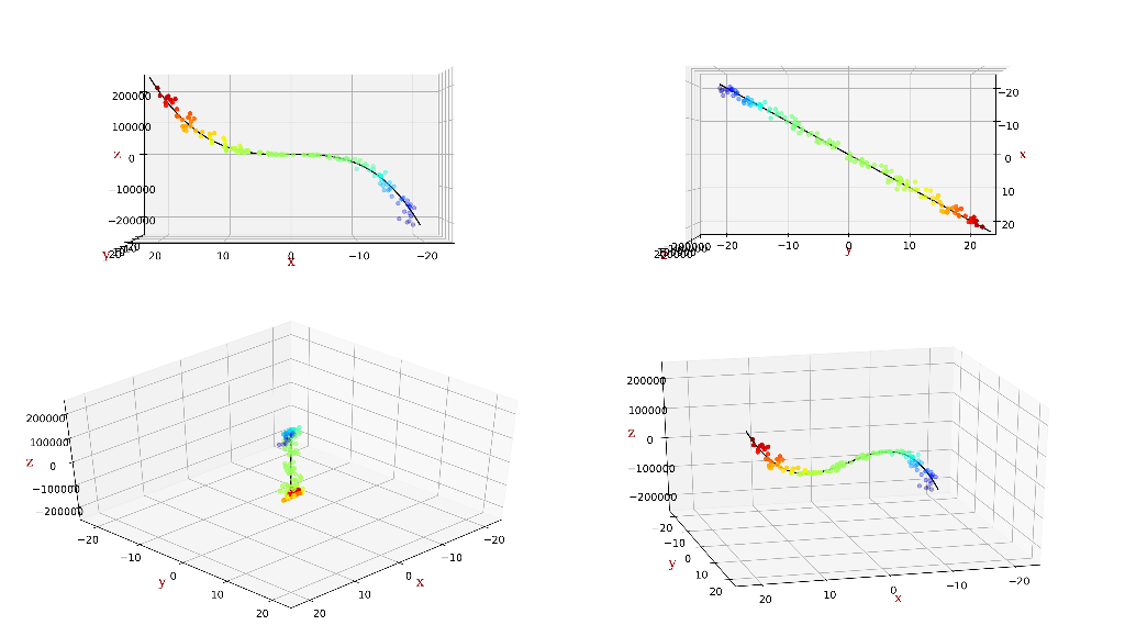
Step by Step Solution
There are 3 Steps involved in it
Step: 1

Get Instant Access to Expert-Tailored Solutions
See step-by-step solutions with expert insights and AI powered tools for academic success
Step: 2

Step: 3
Ace Your Homework with AI
Get the answers you need in no time with our AI-driven, step-by-step assistance
Get Started
Database Systems For Advanced Applications 17th International Conference Dasfaa 2012 International Workshops Flashdb Items Snsm Sim Dqdi Busan South Korea April 2012 Proceedings Lncs 7240
Authors: Hwanjo Yu ,Ge Yu ,Wynne Hsu ,Yang-Sae Moon ,Rainer Unland ,Jaesoo Yoo
2012th Edition
3642290221, 978-3642290220