please help! Thank you!"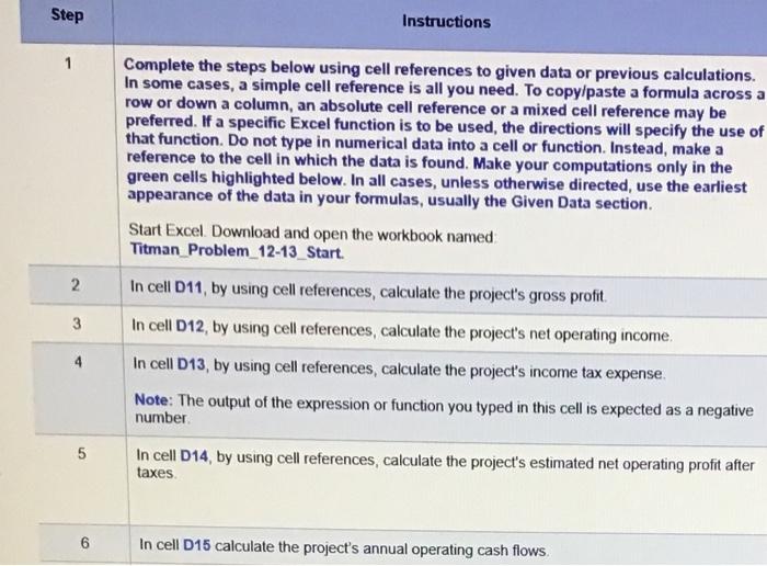

There is nothing missing. This is it. Please respond showing formulas for a thumbs up. Thank you.

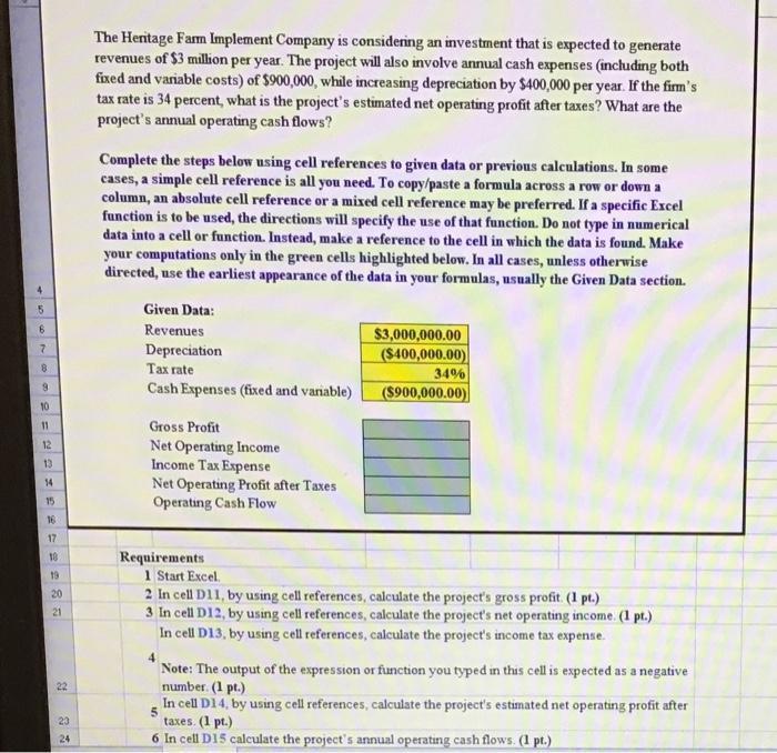
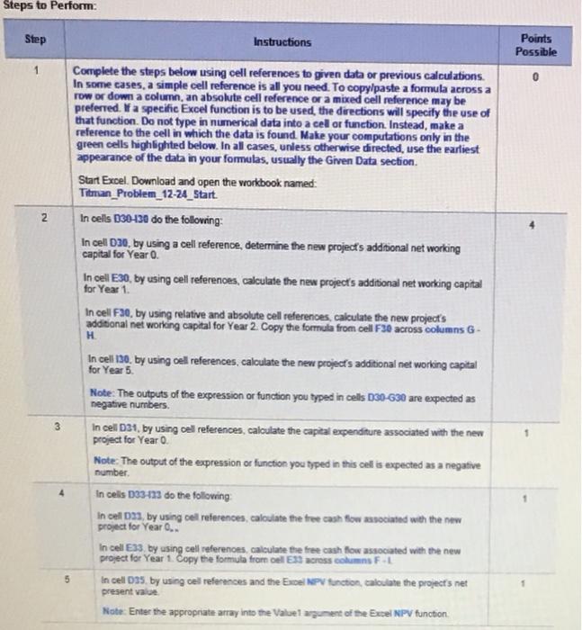
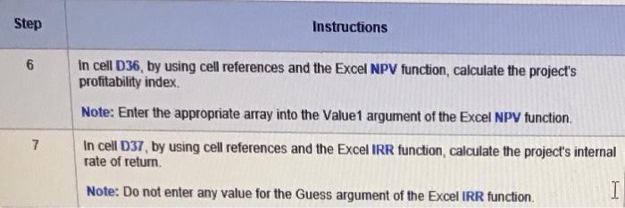
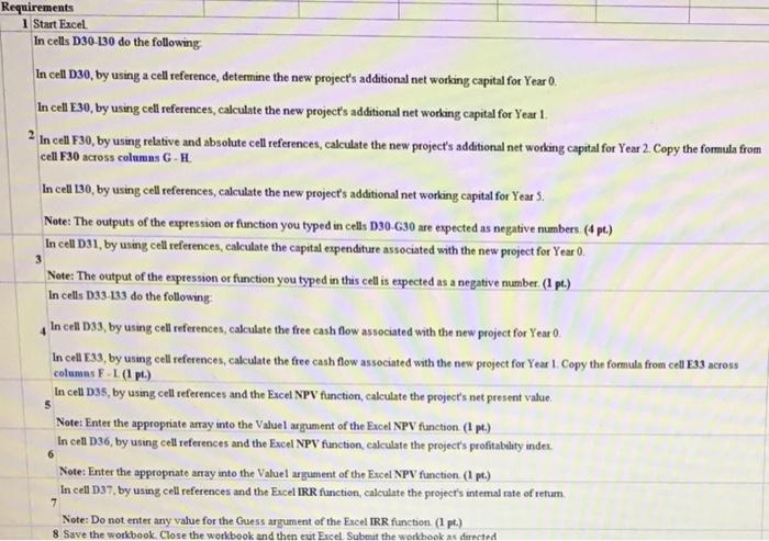
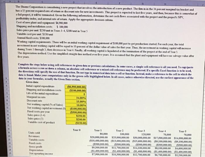
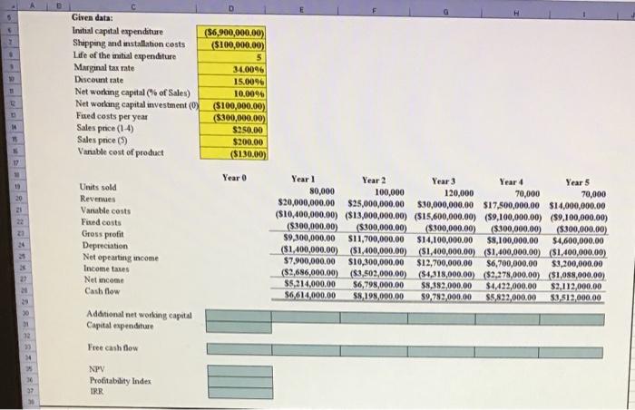
Step Instructions 1 Complete the steps below using cell references to given data or previous calculations. In some cases, a simple cell reference is all you need. To copy/paste a formula across a row or down a column, an absolute cell reference or a mixed cell reference may be preferred. If a specific Excel function is to be used, the directions will specify the use of that function. Do not type in numerical data into a cell or function. Instead, make a reference to the cell in which the data is found. Make your computations only in the green cells highlighted below. In all cases, unless otherwise directed, use the earliest appearance of the data in your formulas, usually the Given Data section. Start Excel. Download and open the workbook named Titman Problem_12-13_Start. In cell D11, by using cell references, calculate the project's gross profit. In cell D12, by using cell references, calculate the project's net operating income In cell D13, by using cell references, calculate the project's income tax expense Note: The output of the expression or function you typed in this cell is expected as a negative number In cell D14, by using cell references, calculate the project's estimated net operating profit after taxes 2. 3 4 5 6 In cell D15 calculate the project's annual operating cash flows. The Henitage Farm Implement Company is considering an investment that is expected to generate revenues of $3 million per year. The project will also involve annual cash expenses (including both fixed and variable costs) of $900,000, while increasing depreciation by $400,000 per year. If the firm's tax rate is 34 percent, what is the project's estimated net operating profit after taxes? What are the project's annual operating cash flows? Complete the steps below using cell references to given data or previous calculations. In some cases, a simple cell reference is all you need. To copy/paste a formula across a row or down a column, an absolute cell reference or a mixed cell reference may be preferred. If a specific Excel function is to be used, the directions will specify the use of that function. Do not type in numerical data into a cell or function. Instead, make a reference to the cell in which the data is found. Make your computations only in the green cells highlighted below. In all cases, unless otherwise directed, use the earliest appearance of the data in your formulas, usually the Given Data section. Given Data: Revenues $3,000,000.00 Depreciation ($400,000.00) Tax rate 34% Cash Expenses (fixed and vanable) ($900,000.00) . 6 7 8 10 11 12 13 Gross Profit Net Operating Income Income Tax Expense Net Operating Profit after Taxes Operating Cash Flow 54 15 16 17 18 19 20 21 Requirements 1 Start Excel 2 In cell D11, by using cell references, calculate the project's gross profit. (1 pt.) 3 In cell D12, by using cell references, calculate the project's net operating income. (1 pt.) In cell D13, by using cell references, calculate the project's income tax expense. 4 Note: The output of the expression or function you typed in this cell is expected as a negative number (1 pt.) In cell D14, by using cell references, calculate the project's estimated net operating profit after taxes (1 pt.) 6 In cell D15 calculate the project's annual operating cash flows (1 pt.) 22 5 23 24 Steps to Perform Step Instructions Points Possible 1 0 2 Complete the steps below using cell references to given data or previous calculations. In some cases, a simple cell reference is all you need. To copy/paste a formula across a row or down a column, an absolute cell reference or a mixed cell reference may be preferred. W a specific Excel function is to be used, the directions will specify the use of that function. Do not type in numerical data into a celor function. Instead, make a reference to the cell in which the data is found. Make your computations only in the green cells highlighted below. In all cases, unless otherwise directed, use the earliest appearance of the data in your formulas, usually the Given Data section. Start Excel. Download and open the workbook named: Titman_Problem_12-24_Start. In cells 030-130 do the following: In cell 030, by using a cell reference, determine the new projects additional net working capital for Year 0. In cell E30, by using cell references, calculate the new project's additional net working capital for Year 1 In cell F30, by using relative and absolute cell references, calculate the new projects additional net working capital for Year 2. Copy the formula from cell F30 across columns G. H In cell 130, by using cell references, calculate the new project's additional net working capital for Year 5. Note: The outputs of the expression or function you typed in cells 030-630 are expected as negative numbers. In cell D31, by using cell references, calculate the capital expenditure associated with the new project for Year 0. Note: The output of the expression or function you typed in this cell is expected as a negative number In cells 103-133 do the following In cell 039, by using cell references, calculate the free cash flow associated with the new project for Year 0.. In cell Es3 by using cell references calculate the free cash flow associated with the new project for Year 1. Copy the formula from del EX cross colons F In cell 035 by using cel references and the Excel NPV function, calculate the project's net present value Note: Enter the appropriate array into the Valve gument of the Excel NPV function 3 1 5 Step Instructions 6 in cell D36, by using cell references and the Excel NPV function, calculate the project's profitability index Note: Enter the appropriate array into the Value1 argument of the Excel NPV function 7 In cell D37, by using cell references and the Excel IRR function, calculate the project's internal rate of return I Note: Do not enter any value for the Guess argument of the Excel IRR function. 3 Requirements 1 Start Excel In cells D30-130 do the following In cell D30, by using a cell reference, determine the new project's additional net working capital for Year 0. In cell E30, by using cell references, calculate the new project's additional net working capital for Year 1. In cell F30, by using relative and absolute cell references, calculate the new project's additional net working capital for Year 2. Copy the formula from cell F30 across columns G-H In cell 130, by using cell references, calculate the new project's additional net working capital for Year 5. Note: The outputs of the expression or function you typed in cells D30-G30 are expected as negative numbers (4 pt.) In cell D31, by using cell references, calculate the capital expenditure associated with the new project for Year 0. Note: The output of the expression or function you typed in this cell is expected as a negative number. (I pt.) In cells D33-133 do the following In cell D33, by using cell references, calculate the free cash flow associated with the new project for Year 0 In cell E33, by using cell references, calculate the free cash flow associated with the new project for Year 1. Copy the formula from cell 33 across columns F-1 (pl.) In cell 035, by using cell references and the Excel NPV function, calculate the project's net present value Note: Enter the appropriate array into the Vabuel argument of the Excel NPV function. (1 pt.) In cell D36, by using cell references and the Excel NPV function calculate the project's profitability index Note: Enter the appropriate array into the Valuel argument of the Excel NPV function (1 pt.) In cell D37, by using cell references and the Excel IRR function calculate the project's intemal rate of retum Note: Do not enter any value for the Guess argument of the Excel IRR function (1 p.) 8 Save the workbook. Close the workbook and then est Excel Submit the workhook as directed 6 7. The Shome Corporation is considering a new project that involves the introduction of a new product. The form in in the 34 percent marginal tax bracket and has a 15 percent required rate of retum or discount rate for new investments. This project is expected to last five years, and then, because thuis is somewhat of a fad project, it will be terminated. Given the following information, determine the net cash flows associated with the project and the project's NPV, profitability index, and internal rate of retum Apply the appropriate decision cntena Cost of new plant and equipment 56,900,000 Shipping and installation costs $ 100,000 Sales pnce per unut: $250/unut in Years 1-4, $200/unit in Year 5 Variable cost per unit: $130/unit Annual fixed costs: $300,000 Working capital requirements: Thete will be an initial working capital requirement of $100,000 just to get production started. For each year, the total wvestment in net working capital will be equal to 10 percent of the dollar value of sales for that year. Thus, the investment in working capital will increase daning Years 1 through 3, then decrease in Year 4 Finally, all working capital is liquidated at the termination of the project at the end of Year The depreciation method. Use the simplified straight line method over five years. It is assumed that the plant and equipment will have no salvage value after five years Complete the steps below using cell references to given data or previons calculations. In some cases, a simple cell reference is all you need. To copy/paste a formula across a row or down a column, an absolute cell reference or a mixed cell reference may be preferred. If a specific Excel function is to be used, the directions will specify the use of that function. Do not type in numerical data into a cell or function. Instead, make a reference to the cell in which the data is found. Make your computations only in the green cells highlighted below. In all cases, unless otherwise directed, use the earliest appearance of the data in your formulas, usually the Given Data section. Given data: Initial capital expenditure ($6.900,000.00) Shipping and installation costs ($100,000.00) Life of the mutual expenditure Marginal tax rate 34.0096 Discount rate 15.0096 Net working capital of Sales) 10.00% Net working capital investment (0) ($100,000.00) Faed costs per year (5300,000.00) Sales pece (14) $250.00 Salespace (5) $200.00 Vanable cost of product ($130.00) Year o Year! Year 2 Year 3 Year 4 Years Units sold 80,000 100,000 120,000 70,000 70,000 Revenues $20,000,000.00 $25,000,000.00 $30,000,000.00 $17.500,000.00 $14,000,000.00 Vanable costs (510.400,000.00) ($13,000,000,00) ($15,600,000,00) (59,100,000.00) (59,100,000.00) Feed costs (5300,000,00) (8.300,000.00 ($100,000,00) (5.300.000,00) (8:300,000.00) Gross profit $9,300,000.00 $11,700,000.00 $14,100,000.00 58,100,000.00 $4,600,000.00 Depreciation ($1,400,000.00 (S1.400,000.00) ($1,400,000,00) 51,400,000,00) 51,400,000.00) Netopearing income $7.900,000.00 $10,300,000.00 $12.700.000,00 56,700,000.00 $3,200,000.00 14 Given data: Initial capital expenditure ($6,900,000.00) Shopping and installation costs ($100,000.00) Life of the initial expenditure Marginal tax rate 34.0096 Discount rate 15.009 Net working capital (% of Sales) 10.0096 Net working capital investment (0) ($100,000.00) Faed costs per year ($300,000.00) Sales price (1-4) $250.00 Sales price (5) $200.00 Vanable cost of product ($130.00) 17 Year 0 19 20 El 22 Units sold Revenues Vanable costs Fed costs Gross profit Depreciation Netopearing income Income taxes Net income Cash flow Year 1 Year 2 Year 3 Year 4 Year 5 80,000 100,000 120,000 70,000 70,000 $20,000,000.00 $25,000,000.00 $30,000,000.00 $17,500,000.00 $14,000,000.00 ($10,400,000.00) ($13,000,000,00) ($15,600,000.00) (59,100,000.00) (89,100,000.00) (8300,000.00) (8.300,000.00) (5300,000.00) ($300,000.00 (5.300,000.00) $9,300,000.00 S11,700,000.00 $14,100,000.00 $8,100,000.00 $4,600,000.00 ($1,400,000.00) ($1,400,000.00) ($1,400,000.00) ($1,400,000.00) ($1,400,000.00) $7,900,000.00 $10,300,000.00 $12,700,000.00 $6,700,000.00 $3,200,000.00 ($2,686,000.00) (83,502,000.00) (54,318,000,00) ($2,278,000.00) ($1,088,000.00) $5,214,000.00 56,798,000.00 $8,182,000,00 $4,422,000.00 $2,112,000.00 $6,614,000.00 $8,198,000.00 59,782,000.00 $5,822,000.00 $3.512,000.00 Additional networking capital Capital expenditure Free cash flow NPV Profitability Index IRR Step Instructions 1 Complete the steps below using cell references to given data or previous calculations. In some cases, a simple cell reference is all you need. To copy/paste a formula across a row or down a column, an absolute cell reference or a mixed cell reference may be preferred. If a specific Excel function is to be used, the directions will specify the use of that function. Do not type in numerical data into a cell or function. Instead, make a reference to the cell in which the data is found. Make your computations only in the green cells highlighted below. In all cases, unless otherwise directed, use the earliest appearance of the data in your formulas, usually the Given Data section. Start Excel. Download and open the workbook named Titman Problem_12-13_Start. In cell D11, by using cell references, calculate the project's gross profit. In cell D12, by using cell references, calculate the project's net operating income In cell D13, by using cell references, calculate the project's income tax expense Note: The output of the expression or function you typed in this cell is expected as a negative number In cell D14, by using cell references, calculate the project's estimated net operating profit after taxes 2. 3 4 5 6 In cell D15 calculate the project's annual operating cash flows. The Henitage Farm Implement Company is considering an investment that is expected to generate revenues of $3 million per year. The project will also involve annual cash expenses (including both fixed and variable costs) of $900,000, while increasing depreciation by $400,000 per year. If the firm's tax rate is 34 percent, what is the project's estimated net operating profit after taxes? What are the project's annual operating cash flows? Complete the steps below using cell references to given data or previous calculations. In some cases, a simple cell reference is all you need. To copy/paste a formula across a row or down a column, an absolute cell reference or a mixed cell reference may be preferred. If a specific Excel function is to be used, the directions will specify the use of that function. Do not type in numerical data into a cell or function. Instead, make a reference to the cell in which the data is found. Make your computations only in the green cells highlighted below. In all cases, unless otherwise directed, use the earliest appearance of the data in your formulas, usually the Given Data section. Given Data: Revenues $3,000,000.00 Depreciation ($400,000.00) Tax rate 34% Cash Expenses (fixed and vanable) ($900,000.00) . 6 7 8 10 11 12 13 Gross Profit Net Operating Income Income Tax Expense Net Operating Profit after Taxes Operating Cash Flow 54 15 16 17 18 19 20 21 Requirements 1 Start Excel 2 In cell D11, by using cell references, calculate the project's gross profit. (1 pt.) 3 In cell D12, by using cell references, calculate the project's net operating income. (1 pt.) In cell D13, by using cell references, calculate the project's income tax expense. 4 Note: The output of the expression or function you typed in this cell is expected as a negative number (1 pt.) In cell D14, by using cell references, calculate the project's estimated net operating profit after taxes (1 pt.) 6 In cell D15 calculate the project's annual operating cash flows (1 pt.) 22 5 23 24 Steps to Perform Step Instructions Points Possible 1 0 2 Complete the steps below using cell references to given data or previous calculations. In some cases, a simple cell reference is all you need. To copy/paste a formula across a row or down a column, an absolute cell reference or a mixed cell reference may be preferred. W a specific Excel function is to be used, the directions will specify the use of that function. Do not type in numerical data into a celor function. Instead, make a reference to the cell in which the data is found. Make your computations only in the green cells highlighted below. In all cases, unless otherwise directed, use the earliest appearance of the data in your formulas, usually the Given Data section. Start Excel. Download and open the workbook named: Titman_Problem_12-24_Start. In cells 030-130 do the following: In cell 030, by using a cell reference, determine the new projects additional net working capital for Year 0. In cell E30, by using cell references, calculate the new project's additional net working capital for Year 1 In cell F30, by using relative and absolute cell references, calculate the new projects additional net working capital for Year 2. Copy the formula from cell F30 across columns G. H In cell 130, by using cell references, calculate the new project's additional net working capital for Year 5. Note: The outputs of the expression or function you typed in cells 030-630 are expected as negative numbers. In cell D31, by using cell references, calculate the capital expenditure associated with the new project for Year 0. Note: The output of the expression or function you typed in this cell is expected as a negative number In cells 103-133 do the following In cell 039, by using cell references, calculate the free cash flow associated with the new project for Year 0.. In cell Es3 by using cell references calculate the free cash flow associated with the new project for Year 1. Copy the formula from del EX cross colons F In cell 035 by using cel references and the Excel NPV function, calculate the project's net present value Note: Enter the appropriate array into the Valve gument of the Excel NPV function 3 1 5 Step Instructions 6 in cell D36, by using cell references and the Excel NPV function, calculate the project's profitability index Note: Enter the appropriate array into the Value1 argument of the Excel NPV function 7 In cell D37, by using cell references and the Excel IRR function, calculate the project's internal rate of return I Note: Do not enter any value for the Guess argument of the Excel IRR function. 3 Requirements 1 Start Excel In cells D30-130 do the following In cell D30, by using a cell reference, determine the new project's additional net working capital for Year 0. In cell E30, by using cell references, calculate the new project's additional net working capital for Year 1. In cell F30, by using relative and absolute cell references, calculate the new project's additional net working capital for Year 2. Copy the formula from cell F30 across columns G-H In cell 130, by using cell references, calculate the new project's additional net working capital for Year 5. Note: The outputs of the expression or function you typed in cells D30-G30 are expected as negative numbers (4 pt.) In cell D31, by using cell references, calculate the capital expenditure associated with the new project for Year 0. Note: The output of the expression or function you typed in this cell is expected as a negative number. (I pt.) In cells D33-133 do the following In cell D33, by using cell references, calculate the free cash flow associated with the new project for Year 0 In cell E33, by using cell references, calculate the free cash flow associated with the new project for Year 1. Copy the formula from cell 33 across columns F-1 (pl.) In cell 035, by using cell references and the Excel NPV function, calculate the project's net present value Note: Enter the appropriate array into the Vabuel argument of the Excel NPV function. (1 pt.) In cell D36, by using cell references and the Excel NPV function calculate the project's profitability index Note: Enter the appropriate array into the Valuel argument of the Excel NPV function (1 pt.) In cell D37, by using cell references and the Excel IRR function calculate the project's intemal rate of retum Note: Do not enter any value for the Guess argument of the Excel IRR function (1 p.) 8 Save the workbook. Close the workbook and then est Excel Submit the workhook as directed 6 7. The Shome Corporation is considering a new project that involves the introduction of a new product. The form in in the 34 percent marginal tax bracket and has a 15 percent required rate of retum or discount rate for new investments. This project is expected to last five years, and then, because thuis is somewhat of a fad project, it will be terminated. Given the following information, determine the net cash flows associated with the project and the project's NPV, profitability index, and internal rate of retum Apply the appropriate decision cntena Cost of new plant and equipment 56,900,000 Shipping and installation costs $ 100,000 Sales pnce per unut: $250/unut in Years 1-4, $200/unit in Year 5 Variable cost per unit: $130/unit Annual fixed costs: $300,000 Working capital requirements: Thete will be an initial working capital requirement of $100,000 just to get production started. For each year, the total wvestment in net working capital will be equal to 10 percent of the dollar value of sales for that year. Thus, the investment in working capital will increase daning Years 1 through 3, then decrease in Year 4 Finally, all working capital is liquidated at the termination of the project at the end of Year The depreciation method. Use the simplified straight line method over five years. It is assumed that the plant and equipment will have no salvage value after five years Complete the steps below using cell references to given data or previons calculations. In some cases, a simple cell reference is all you need. To copy/paste a formula across a row or down a column, an absolute cell reference or a mixed cell reference may be preferred. If a specific Excel function is to be used, the directions will specify the use of that function. Do not type in numerical data into a cell or function. Instead, make a reference to the cell in which the data is found. Make your computations only in the green cells highlighted below. In all cases, unless otherwise directed, use the earliest appearance of the data in your formulas, usually the Given Data section. Given data: Initial capital expenditure ($6.900,000.00) Shipping and installation costs ($100,000.00) Life of the mutual expenditure Marginal tax rate 34.0096 Discount rate 15.0096 Net working capital of Sales) 10.00% Net working capital investment (0) ($100,000.00) Faed costs per year (5300,000.00) Sales pece (14) $250.00 Salespace (5) $200.00 Vanable cost of product ($130.00) Year o Year! Year 2 Year 3 Year 4 Years Units sold 80,000 100,000 120,000 70,000 70,000 Revenues $20,000,000.00 $25,000,000.00 $30,000,000.00 $17.500,000.00 $14,000,000.00 Vanable costs (510.400,000.00) ($13,000,000,00) ($15,600,000,00) (59,100,000.00) (59,100,000.00) Feed costs (5300,000,00) (8.300,000.00 ($100,000,00) (5.300.000,00) (8:300,000.00) Gross profit $9,300,000.00 $11,700,000.00 $14,100,000.00 58,100,000.00 $4,600,000.00 Depreciation ($1,400,000.00 (S1.400,000.00) ($1,400,000,00) 51,400,000,00) 51,400,000.00) Netopearing income $7.900,000.00 $10,300,000.00 $12.700.000,00 56,700,000.00 $3,200,000.00 14 Given data: Initial capital expenditure ($6,900,000.00) Shopping and installation costs ($100,000.00) Life of the initial expenditure Marginal tax rate 34.0096 Discount rate 15.009 Net working capital (% of Sales) 10.0096 Net working capital investment (0) ($100,000.00) Faed costs per year ($300,000.00) Sales price (1-4) $250.00 Sales price (5) $200.00 Vanable cost of product ($130.00) 17 Year 0 19 20 El 22 Units sold Revenues Vanable costs Fed costs Gross profit Depreciation Netopearing income Income taxes Net income Cash flow Year 1 Year 2 Year 3 Year 4 Year 5 80,000 100,000 120,000 70,000 70,000 $20,000,000.00 $25,000,000.00 $30,000,000.00 $17,500,000.00 $14,000,000.00 ($10,400,000.00) ($13,000,000,00) ($15,600,000.00) (59,100,000.00) (89,100,000.00) (8300,000.00) (8.300,000.00) (5300,000.00) ($300,000.00 (5.300,000.00) $9,300,000.00 S11,700,000.00 $14,100,000.00 $8,100,000.00 $4,600,000.00 ($1,400,000.00) ($1,400,000.00) ($1,400,000.00) ($1,400,000.00) ($1,400,000.00) $7,900,000.00 $10,300,000.00 $12,700,000.00 $6,700,000.00 $3,200,000.00 ($2,686,000.00) (83,502,000.00) (54,318,000,00) ($2,278,000.00) ($1,088,000.00) $5,214,000.00 56,798,000.00 $8,182,000,00 $4,422,000.00 $2,112,000.00 $6,614,000.00 $8,198,000.00 59,782,000.00 $5,822,000.00 $3.512,000.00 Additional networking capital Capital expenditure Free cash flow NPV Profitability Index IRR