please help these are the steps

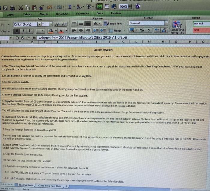
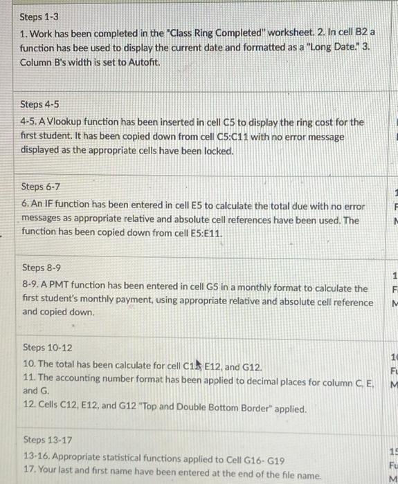
2.2. Y 100% Number Format General Normal Layout Tables Charts SmartArt Formula Data Raview Font Alignment Fill Calibri (Body) AA- abc- Wrap Text Clear B 7 U Merge fx Adapted from 2017 Pearson Microsoft Office 2016 V.1 Grauer B 6.0 03 0.0 ES Conditional Formatting Bad M N Custom Jewelers Custom Jewelers makes custom class rings for graduating seniors. As an accounting manager you want to create a workbook to report details on total costs to the student as well as payment Information. Each ring financed has a base price plus ding personlization 1. The "Cats Ring Raw Data tab" contains all of the information to complete the exercise. Creat a copy of this worksheet and label it "Class Ring Completed." All of your work should be completed in the Completed tah. 2. In cell 2 inserta function to display the current date and format it as a long Date 3. Set 's width to Autofit. You will calculate the cost of each class ring ordered. The rings are priced based on their base metal displayed in the range A15.819 4. Insert a Vlookup function in cell CS to display the ring cost for the first student 5 Copy the function from cell cs down through 11 to complete column C. Ensure the appropriate cells are lacked or else the formula will not autofill properly. Glance over the information that has been filled in mange CS to Cut to ensure it appropriately corresponds with base metal displayed in the range 15:019. You will calculate the total due for each student's order. The total is the base price of the ring plus an additional change for personalization if applicable. 6. Insert an IF function in cells to calculate the total due. If the student has chosen to personline the ring tas indicated in column D), there is an additional charge of 6% located in colla21 that must be applied. If not, the student only pays the base price. Note that when entering text in your formulation you must put quotation marks before and after it lle"Yes"). Use appropriate relative and absolute cell references. 7. Copy the function from cells down through 11. The next step is to calitate the periodic payment for each student's account. The payments we based on the years financed in column and the annual intereste rate in cell 122. All accounts are paid on a monthly basis 3. Insert a PMT function in cells to calculate the first student's monthly payment, utine propriate relative and absolute cell reference Ensure that all information is provided monthly under "Monthly Payment as the interest rate and the years financed are provided in a yearly format 9. Copy the formula down the column 10. Calculate the total in cel C12, E12, and G12 11. Apply the accounting number format to decimal places for column., and G. 12. In cells 612, E12, and 612 apply "Top and Double Bottom Border for the totals. 11. In cell G16 apply a statistical function calculating the average monthly payment Per Customer for Inland Jewiers Instructions Class Ring Raw Data Normal View Ready Steps 1-3 1. Work has been completed in the "Class Ring Completed" worksheet. 2. In cell B2 a function has bee used to display the current date and formatted as a "Long Date. 13. Column B's width is set to Autofit. Steps 4-5 4-5. A Vlookup function has been inserted in cell C5 to display the ring cost for the first student. It has been copied down from cell C5:C11 with no error message displayed as the appropriate cells have been locked. Steps 6-7 6. An IF function has been entered in cell E5 to calculate the total due with no error messages as appropriate relative and absolute cell references have been used. The function has been copied down from cell E5:E11. N Steps 8-9 8-9. A PMT function has been entered in cell G5 in a monthly format to calculate the first student's monthly payment, using appropriate relative and absolute cell reference and copied down F Steps 10-12 10. The total has been calculate for cell C1 E12, and G12. 11. The accounting number format has been applied to decimal places for column C, E, and G. 12. Cells C12, E12, and G12 "Top and Double Bottom Border" applied. Steps 13-17 13-16. Appropriate statistical functions applied to Cell G16 G19 17. Your last and first name have been entered at the end of the file name. 19 Fu M 2.2. Y 100% Number Format General Normal Layout Tables Charts SmartArt Formula Data Raview Font Alignment Fill Calibri (Body) AA- abc- Wrap Text Clear B 7 U Merge fx Adapted from 2017 Pearson Microsoft Office 2016 V.1 Grauer B 6.0 03 0.0 ES Conditional Formatting Bad M N Custom Jewelers Custom Jewelers makes custom class rings for graduating seniors. As an accounting manager you want to create a workbook to report details on total costs to the student as well as payment Information. Each ring financed has a base price plus ding personlization 1. The "Cats Ring Raw Data tab" contains all of the information to complete the exercise. Creat a copy of this worksheet and label it "Class Ring Completed." All of your work should be completed in the Completed tah. 2. In cell 2 inserta function to display the current date and format it as a long Date 3. Set 's width to Autofit. You will calculate the cost of each class ring ordered. The rings are priced based on their base metal displayed in the range A15.819 4. Insert a Vlookup function in cell CS to display the ring cost for the first student 5 Copy the function from cell cs down through 11 to complete column C. Ensure the appropriate cells are lacked or else the formula will not autofill properly. Glance over the information that has been filled in mange CS to Cut to ensure it appropriately corresponds with base metal displayed in the range 15:019. You will calculate the total due for each student's order. The total is the base price of the ring plus an additional change for personalization if applicable. 6. Insert an IF function in cells to calculate the total due. If the student has chosen to personline the ring tas indicated in column D), there is an additional charge of 6% located in colla21 that must be applied. If not, the student only pays the base price. Note that when entering text in your formulation you must put quotation marks before and after it lle"Yes"). Use appropriate relative and absolute cell references. 7. Copy the function from cells down through 11. The next step is to calitate the periodic payment for each student's account. The payments we based on the years financed in column and the annual intereste rate in cell 122. All accounts are paid on a monthly basis 3. Insert a PMT function in cells to calculate the first student's monthly payment, utine propriate relative and absolute cell reference Ensure that all information is provided monthly under "Monthly Payment as the interest rate and the years financed are provided in a yearly format 9. Copy the formula down the column 10. Calculate the total in cel C12, E12, and G12 11. Apply the accounting number format to decimal places for column., and G. 12. In cells 612, E12, and 612 apply "Top and Double Bottom Border for the totals. 11. In cell G16 apply a statistical function calculating the average monthly payment Per Customer for Inland Jewiers Instructions Class Ring Raw Data Normal View Ready Steps 1-3 1. Work has been completed in the "Class Ring Completed" worksheet. 2. In cell B2 a function has bee used to display the current date and formatted as a "Long Date. 13. Column B's width is set to Autofit. Steps 4-5 4-5. A Vlookup function has been inserted in cell C5 to display the ring cost for the first student. It has been copied down from cell C5:C11 with no error message displayed as the appropriate cells have been locked. Steps 6-7 6. An IF function has been entered in cell E5 to calculate the total due with no error messages as appropriate relative and absolute cell references have been used. The function has been copied down from cell E5:E11. N Steps 8-9 8-9. A PMT function has been entered in cell G5 in a monthly format to calculate the first student's monthly payment, using appropriate relative and absolute cell reference and copied down F Steps 10-12 10. The total has been calculate for cell C1 E12, and G12. 11. The accounting number format has been applied to decimal places for column C, E, and G. 12. Cells C12, E12, and G12 "Top and Double Bottom Border" applied. Steps 13-17 13-16. Appropriate statistical functions applied to Cell G16 G19 17. Your last and first name have been entered at the end of the file name. 19 Fu M


