Please help verify formulas are correct.

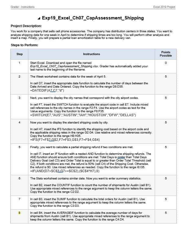
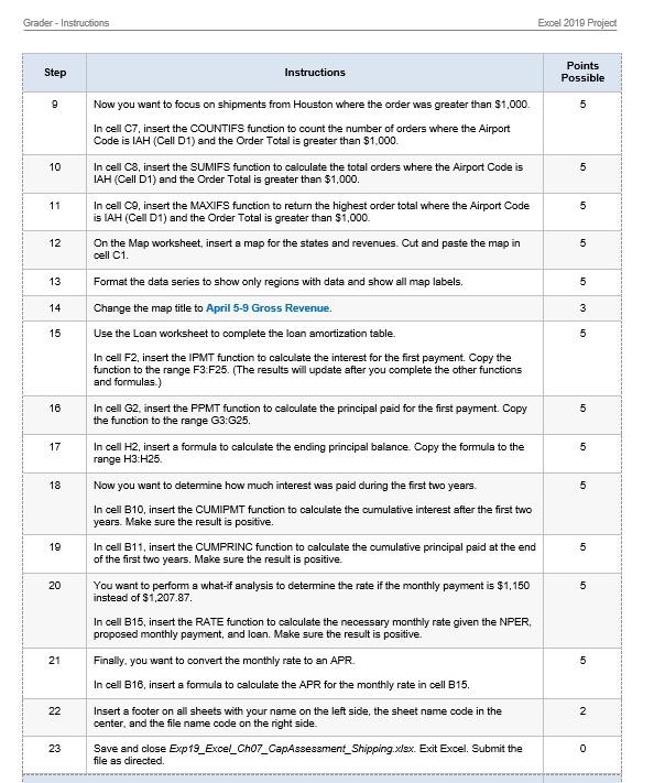
Instructions in this link:

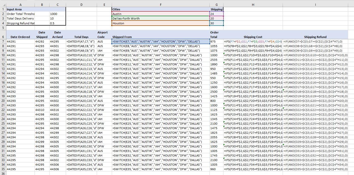
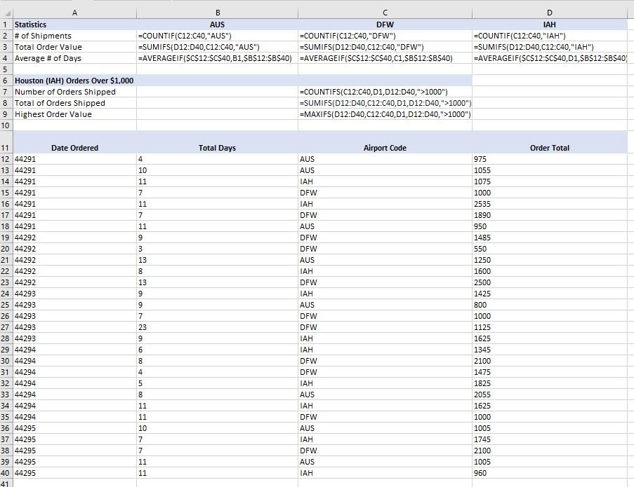
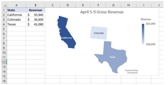
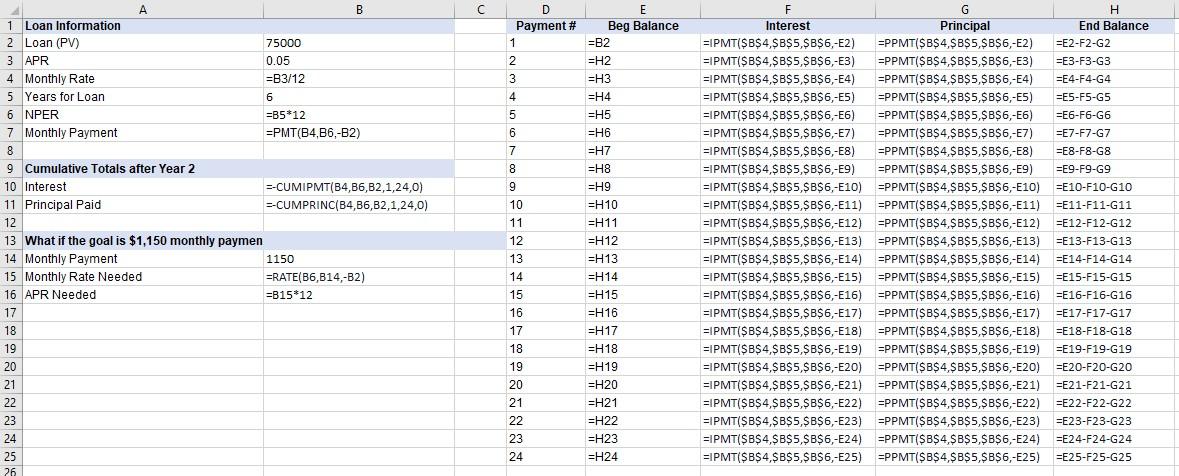
C D E F H 1000 10 0.5 cities Austin Dallas-Forth Worth [ Houston G Shipping! 24 120 30 Date Arrived 44295 44301 44302 44298 44302 44298 44302 44301 A B 1 Input Area 2 Order Total Thresho 3 Total Days Delivery 4 Shipping Refund Rat 5 Date 6 Date Ordered Shipped 7 44291 44292 8 44291 44293 9 44291 44293 10 44291 44293 11 44291 44295 12 44291 44291 13 44291 44294 14 44292 44294 15 44292 44292 16 44292 44294 17 44292 44294 18 44292 44295 19 44293 44298 20 44293 44295 21 44293 44295 22 44293 44310 23 44293 44298 24 44294 44295 25 44294 44295 26 44294 44294 27 44294 44295 28 44294 44298 29 44294 44299 30 44294 44298 31 44295 44298 32 44295 44298 33 44295 44298 34 44295 44295 35 44295 44295 36 44295 44305 44300 44305 44302 44302 Airport Total Days Code =DATEDIF(A7,c7,"d") AUS =DATEDIF(A8,C8,"d") AUS =DATEDIF(A9,C9,"d") IAH =DATEDIF(A10,010,"d" DFW =DATEDIF(A11,011,"d"IAH =DATEDIF(A12,012,"d" DFW =DATEDIF(A13,C13,"d" AUS EDATEDIF(A14,C14,"d" DFW EDATEDIF(A15,C15,"d" DFW =DATEDIF(A16,C16,"d" AUS =DATEDIF(A17,017,"d" IAH =DATEDIF(A18,C18,"d" DFW =DATEDIF(A19, C19,"d" IAH =DATEDIF(A20,020,"d" AUS =DATEDIF(A21,C21,"d" DFW =DATEDIF(A22,222,"d" DFW =DATEDIF(A23,C23,"d" IAH =DATEDIF(A24,024,"d"IAH =DATEDIF(A25,C25,"d" DFW =DATEDIF(A26, C26,"d" DFW =DATEDIF(A27,027,"d"IAH =DATEDIF(A28,C28,"d" AUS =DATEDIF(A29,029,"d" IAH =DATEDIF(A30, C30,"d" DFW =DATEDIF(A31,C31,"d" AUS =DATEDIF(A32,032,"d" IAH =DATEDIF(A33,C33,"d" DFW =DATEDIF(A34,C34,"d" AUS =DATEDIF(A35,035,"d" IAH Shipped From I=SWITCH(E7,"AUS","AUSTIN","IAH","HOUSTON","DFW","DELLAS") =SWITCH(E8,"AUS", "AUSTIN", "IAH", "HOUSTON","DFW","DELLAS") =SWITCH(E9,"AUS", "AUSTIN","IAH","HOUSTON","DFW","DELLAS") =SWITCH(E10,"AUS", "AUSTIN", "IAH","HOUSTON","DFW","DALLAS") =SWITCH(E11,"AUS","AUSTIN","IAH","HOUSTON","DFW","DALLAS") =SWITCH(E12,"AUS","AUSTIN","IAH","HOUSTON","DFW","DALLAS") =SWITCH(E13,"AUS","AUSTIN","IAH","HOUSTON","DFW","DALLAS") =SWITCH(E14,"AUS","AUSTIN","IAH","HOUSTON","DFW","DALLAS") =SWITCH(E15,"AUS","AUSTIN","IAH","HOUSTON","DFW","DALLAS") =SWITCH(E16,"AUS", "AUSTIN","IAH","HOUSTON","DFW","DALLAS") =SWITCH(E17,"AUS","AUSTIN","IAH","HOUSTON","DFW","DALLAS") =SWITCH(E18,"AUS", "AUSTIN","IAH","HOUSTON","DFW","DALLAS") =SWITCH(E19,"AUS", "AUSTIN","IAH", "HOUSTON","DFW","DALLAS") =SWITCH(E20,"AUS","AUSTIN","IAH","HOUSTON","DFW","DALLAS") =SWITCH(E21,"AUS","AUSTIN","IAH","HOUSTON","DFW","DALLAS") =SWITCH(E22,"AUS","AUSTIN","IAH","HOUSTON","DFW","DALLAS") =SWITCH(E23,"AUS","AUSTIN","IAH", "HOUSTON","DFW","DALLAS") =SWITCH(E24,"AUS","AUSTIN", "IAH","HOUSTON","DFW","DALLAS") =SWITCH(E25,"AUS", "AUSTIN","IAH","HOUSTON","DFW","DALLAS") =SWITCH(E26,"AUS","AUSTIN","IAH","HOUSTON","DFW","DALLAS") =SWITCH(E27,"AUS","AUSTIN", "IAH","HOUSTON","DFW","DALLAS") =SWITCH(E28,"AUS","AUSTIN","IAH","HOUSTON","DFW","DALLAS") =SWITCH(E29,"AUS","AUSTIN","IAH","HOUSTON","DFW","DALLAS") =SWITCH(E30,"AUS", "AUSTIN","IAH","HOUSTON","DFW","DALLAS") =SWITCH(E31,"AUS","AUSTIN","IAH","HOUSTON","DFW","DALLAS") =SWITCH(E32,"AUS","AUSTIN", "IAH","HOUSTON","DFW","DALLAS") =SWITCH(E33,"AUS","AUSTIN","IAH","HOUSTON","DFW","DALLAS") =SWITCH(E34,"AUS", "AUSTIN","IAH","HOUSTON","DFW","DALLAS") =SWITCH(E35,"AUS","AUSTIN","IAH","HOUSTON","DFW","DALLAS") Order Total 1975 1055 1075 1000 2535 1890 950 1485 550 1250 1600 2500 1425 800 1000 1125 1625 1345 2100 1475 1825 2055 1625 1000 1005 1745 2100 1005 960 Shipping Cost Shipping Refund =IFS(F7=F$2,6$2,F7=F$3,6$3,F7=F$ 4,6$ 4) =IF(AND(D7>$C$3,67>=$C$2),($C$4*H7),O) =IFS(F8=F$2,6$2,F8=F$3,6$3,F8=F$ 4,6$4) =IF(AND(D8>$C$3,68>=$C$2),($C$4*H8),0) =IFS(F9=F$2,6$2,F9=F$3,6$3,F9=F$4, G$4) =IF(AND(D9>$C$3,69x=$C$2),($C$4*H9),0) SIFS(F10=F$2,6$2,F10=F$3,6$3,F10=F$4,6 =IF(AND(D10>$C$3,610>=$C$2),($C$4*H10),0) =IFS(F11=F$2,6$2,F11=F$3,6$3,F11=F$4, G EIF(AND(D11>$C$3,611>$C$2),($C$4*H11),0) =IFS(F12=F$2,6$2,F12=F$3,G$3,F12=F$4,6 =IF(AND(D12>$C$3,612>=$C$2),($C$4*H12),0) =IFS(F13=F$2,6$2,F13=F$3,6$3,F13=F$4,6 =IF(AND(D13>$C$3,613>=$C$2),($C$4*H13),0) =IFS(F14=F$2,6$2,F14=F$3,6$3,F14=F$4,6 =IF(AND(014>$C$3,614>=$C$2),($C$4*H14),0) =IFS(F15=F$2,6$2,F15=F$3,6$3,F15=F$4,G EIF(AND(D15>$C$3,615>=$C$2),($C$4*H15),0) =IFS(F16=F$2,G$2,F16=F$3,6$3,F16=F$ 4, G =IF(AND(D16>$C$3,616>=$C$2),($C$4*H16),0) =IFS(F17=F$2,6$2,F17=F$3,6$3,F17=F$4,G =IF(AND(D17>$C$3,617>$C$2),($C$4*H17),0) =IFS(F18=F$2,6$2,F18=F$3,6$3,F18=F$4, G'FIF(AND(D18>$C$3,618>=$C$2),($C$ 4*H18),0) =IFS(F19=F$2,6$2,F19=F$3,6$3,F19=F$4,6 =IF(AND(D19>$C$3,619>$C$2),($C$4*H19),0) =IFS(F20=F$2,G$2,F20=F$3,6$3,F20=F$ 4, G =IF(AND(D20>$C$3,G20>$C$2),($C$4*H20),0) SIFS(F21=F$2,6$2,F21=F$3,6$3,F21=F$4,G EIF(AND(D21>$C$3,621>=$C$2),($C$4*H21),0) =IFS(F22=F$2,G$2,F22=F$3,6$3,F22=F$4,G'=IF(AND(D22>$C$3,622>=$C$2),($C$ 4*H22),0) =IFS(F23=F$2,G$2,F23=F$3,6$3,F23=F$4, G =IF(AND(D23>$C$3,623>$C$2),($c$4*H23),0) =IFS(F24=F$2,6$2,F24=F$3,6$3,F24=F$4,6 =IF(AND(D24>$C$3,624>=$C$2),($C$4*H24),0) =IFS(F25=F$2,G$2,F25=F$3,6$3,F25=F$ 4, G =IF(AND(D25>$C$3,625>$C$2),($C$4*H25),0) =IFS(F26=F$2,6$2,F26=F$3,6$3,F26=F$4, G EIF(AND(D26>$C$3,626>=$C$2),($C$4*H26),0) =IFS(F27=F$2,6$2,F27=F$3,6$3,F27=F$4, G EIF(AND(D27>$C$3,627>=$C$2),($C$4*H27),0) =IFS(F28=F$2,6$2,F28=F$3,6$3,F28=F$4, G =IF(AND(D28>$C$3,628>=$C$2),($C$4*H28),0) =IFS(F29=F$2,G$2,F29=F$3,6$3,F29=F$4,6 =IF(AND(D29>$C$3,629>=$C$2),($C$4*H29),0) =IFS(F30=F$2,G$2,F30=F$3,6$3,F30=F$ 4,G=IF(AND(D30>$C$3,630>=$C$2),($C$4*H30),0) =IFS(F31=F$2,6$2,F31=F$3,6$3,F31=F$4, G EIF(AND(D31>$C$3,631>=$C$2),($C$4*H31),0) =IFS(F32=F$2,G$2,F32=F$3,6$3,F32=F$4,G EIF(AND(D32>$C$3,632>=$C$2),($C$4*H32),0) =IFS(F33=F$2,G$2,F33=F$3,6$3,F33=F$ 4, G =IF(AND(D33>$C$3,633>$C$2),($C$4*H33),0) =IFS(F34=F$2,6$2,F34=F$3,6$3,F34=F$ 4,6 =IF(AND(D34>$C$3,634>$C$2),($C$4*H34),0) =IFS(F35=F$2,6$2,F35=F$3,6$3,F35=F$4, G =IF(AND(D35>$C$3,635>$C$2),($C$4*H35),0) 44300 44316 44302 44300 44302 44298 44299 44302 44305 44305 44305 44302 44302 44306 44306 D B C AUS DFW =COUNTIF(C12:040,"AUS") =COUNTIF(C12:040,"DFW") =SUMIFS(D12:D40,012:040,"AUS") =SUMIFS(D12:040,012:C40,"DFW") =AVERAGEIF($C$12:$C$40,81,$B$12:$B$40) =AVERAGEIF($C$12:$C$40,C1,$B$12:$B$40) =COUNTIF(C12:C40,"IAH") =SUMIFS(D12:D40,C12:040,"AH") =AVERAGEIF($C$12:$C$40,01,$B$12:$B$40! 1 Statistics 2 # of Shipments 3 Total Order Value 4 Average # of Days 5 6 Houston (IAH) Orders Over $1,000 7 Number of Orders Shipped 8 Total of Orders Shipped 9 Highest Order Value 10 =COUNTIFS(C12:040,D1,D12:040,">1000") =SUMIFS(D12:040,C12:040,D1,D12:040,">1000") =MAXIFS(D12:040,012:040,D1,D12:040,">1000") Date Ordered Total Days Airport Code Order Total 4 10 11 7 11 7 11 9 3 13 8 13 9 9 11 12 44291 13 44291 14 44291 15 44291 16 44291 17 44291 18 44291 19 44292 20 44292 21 44292 22 44292 23 44292 24 44293 25 44293 26 44293 27 44293 28 44293 29 44294 30 44294 31 44294 32 44294 33 44294 34 44294 35 44294 36 44295 37 44295 38 44295 39 44295 40 44295 41 7 23 9 6 8 4 5 8 11 11 10 7 7 11 11 AUS AUS IAH DFW IAH DFW AUS DFW DFW AUS IAH DFW IAH AUS DFW DFW IAH IAH DFW DFW IAH AUS IAH DFW AUS IAH DFW AUS IAH 975 1055 1075 1000 2535 1890 950 1485 550 1250 1600 2500 1425 800 1000 1125 1625 1345 2100 1475 1825 2055 1625 1000 1005 1745 2100 1005 960 A D E F G H April 5-9 Gross Revenue 1 State 2 California 3 Colorado 4 Texas 5 B Revenue $ 55,945 $ 30,650 $ 41,080 Revenue $55,945 Colorado 6 7 California $30,650 10 11 12 Texas Powered by Wine GeoNames 15 16 c D Payment # 1 1 2 3 4 5 6 7 8 9 E Beg Balance =B2 =H2 =H3 =H4 =H5 =H6 =H7 =H8 =H9 =H10 A B 1 Loan Information 2 Loan (PV) 75000 3 APR 0.05 4 Monthly Rate =B3/12 5 Years for Loan 6 6 NPER =B5*12 7 Monthly Payment =PMT(B4,B6,-B2) 8 9 Cumulative Totals after Year 2 10 Interest --CUMIPMT(B4,B6,B2,1,24,0) 11 Principal Paid --CUMPRINC(B4,B6,B2,1,24,0) 12 13 What if the goal is $1,150 monthly paymen 14 Monthly Payment 1150 15 Monthly Rate Needed ERATE(B6,B14,-B2) 16 APR Needed =B15 12 17 18 19 20 21 22 23 24 25 26 10 11 12 13 14 15 F G H Interest Principal End Balance =IPMT($B$4,$B$ 5,$B$6,-E2) =PPMT($B$4,$B$5,$B$6,-E2) =E2-F2-G2 =IPMT($B$4,$B$5,$B$6,-E3) =PPMT($B$4, $B$5,$B$ 6,-E3) =E3-F3-G3 =IPMT($B$4,$B$5,$B$6,-E4) =PPMT($B$4.$B$5,$B$ 6,-E4) =E4-F4-G4 =IPMT($B$4,$B$5,$B$6,-E5) =PPMT($B$4,$B$5,$B$ 6,-ES) =E5-F5-G5 =IPMT($B$4,$B$5,$B$6,-E6) =PPMT($B$ 4,$B$5,$B$6,-E6) =E6-F6-G6 =IPMT($B$4,$B$ 5,$B$6,-E7) =PPMT($B$4,$B$5,$B$6,-E7) =E7-F7-G7 =IPMT($B$ 4,$B$5,$B$6,-E8) =PPMT($B$4:$B$5,$B$6,-E8) =E8-F8-G8 =IPMT($B$4,$B$5,$B$ 6,-E9) =PPMT($B$4,$B$5,$B$ 6,-E9) =E9-F9-G9 =IPMT($B$ 4,$B$5,$B$6,-E10) =PPMT($B$ 4,$B$5,$B$ 6,-E10) =E10-F10-G10 =IPMT($B$4,$B$5,$B$ 6,-E11) =PPMT($B$4,$B$5,$B$6,-E11) =E11-F11-G11 =IPMT($B$4,$B$5,$B$6,-E12) =PPMT($B$4:$B$5,$B$ 6,-E12) =E12-F12-G12 =IPMT($B$4,$B$5,$B$ 6,-E13) =PPMT($B$4:$B$5,$B$ 6,-E13) =E13-F13-G13 =IPMT($B$4,$B$5,$B$6,-E14) =PPMT($B$4,$B$5,$B$6,-E14) =E14-F14-G14 =IPMT($B$4,$B$5,$B$ 6,-E15) =PPMT($B$4,$B$5,$B$ 6,-E15) =E15-F15-G15 =IPMT($B$4,$B$5,$B$ 6,-E16) =PPMT($B$4:$B$5,$B$6,-E16) =E16-F16-316 =IPMT($B$4,$B$5,$B$6,-E17) =PPMT($B$4,$B$5,$B$ 6,-E17) B) =E17-F17-G17 =IPMT($B$4,$B$5,$B$ 6,-E18) =PPMT($B$4,$B$5,$B$6,-E18) =B$$B5=E18-F18-618 =IPMT($B$4,$B$5,$B$ 6,-E19) =PPMT($B$4,$B$5,$B$6,-E19) =E19-F19-G19 =IPMT($B$4,$B$5,$B$6,-E20) =PPMT($B$4:$B$5,$B$6,-E20) =E20-F20-G20 =IPMT($B$4,$B$5,$B$ 6,-E21) =PPMT($B$4,$B$5,$B$6,-E21) =E21-F21-G21 =IPMT($B$4,$B$5,$B$6,-E22) =PPMT($B$4,$B$5,$B$ 6,-E22) =E22-F22-22 =IPMT($B$4,$B$5,$B$ 6,-E23)=PPMT($B$4:$B$5,$B$6,-E23) =E23-F23-G23 =IPMT($B$4,$B$5,$B$6,-E24) =PPMT($B$4$B$5,$B$6,-E24) =E24-F24-G24 =IPMT($B$4,$B$5,$B$ 6,-E25) =PPMT($B$4,$B$5,$B$6,-E25) =E25-F25-G25 16 =H11 =H12 =H13 =H14 =H15 =H16 =H17 =H18 =H19 =H20 =H21 =H22 =H23 =H24 17 18 19 20 21 22 23 24 Grader - Instructions Excel 2019 Project Exp19_Excel_Ch07_CapAssessment_Shipping Project Description: You work for a company that sells cell phone accessories. The company has distribution centers in three states. You want to analyze shipping data for one week in April to determine if shipping times are too long. You will perform other analysis and insert a map. Finally, you will prepare a partial loan amortization table for a new delivery van. Steps to Perform: Step Instructions Points Possible 1 0 2 5 3 5 5 Start Excel. Download and open the file named Exp19_Excel_Chor_CapAssessment_Shipping.xlsx. Greder has automatically added your last name to the beginning of the filename. The Week worksheet contains data for the week of April 5. In cell D7, insert the appropriate date function to calculate the number of days between the Date Arrived and Date Ordered. Copy the function to the range DS:D35. =DATEDIF(AZ C7,"d") Next, you want to display the city names that correspond with the city airport codes. In cell F7, insert the SWITCH function to evaluate the airport code in cell E7. Include mixed cell references to the city names in the range F2:F4. Use the airport codes as text for the Value arguments. Copy the function to the range F8:F35. =SWITCH(E7 "AUS", "AUSTIN", "IAH","HOUSTON", "DFW", "DELLAS") Now you want to display the standard shipping costs by city. In cell H7, insert the IFS function to identify the shipping cost based on the airport code and the applicable shipping rates in the range G2:G4. Use relative and mixed references correctly Copy the function to the range H8:H35. =IFS(F7=F$2G$2,F7=F$3,6$3,F7=F$4,G$4) Finally, you want to calculate a partial shipping refund if two conditions are met. In cell 17. insert an IF function with a nested AND function to determine shipping refunds. The AND function should ensure both conditions are met Total Days is grater than Total Days Delivery Goal (cell C3) and Order Total is equal to or greater than Order Total Threshold (cell C2). If both conditions are met, the refund is 50% (cell C4) of the Shipping Cost. Otherwise. the refund is $0. Use mixed references as needed. Copy the function to the range 18:135. =IF(AND(D7>$C$3.G7>=$C$2),($C$4*H7),0) The Stats worksheet contains similar data. Now you want to enter summary statistics. In cell B2, insert the COUNTIF function to count the number of shipments for Austin (cell B1). Use appropriate mixed references to the range argument to keep the column letters the same. Copy the function to the range C2:D2. In cell B3, insert the SUMIF function to calculate the total orders for Austin (cell B1). Use appropriate mixed references to the range argument to keep the column letters the same. Copy the function to the range C3.03. In cell B4, insert the AVERAGEIF function to calculate the average number of days for shipments from Austin (cell B1). Use appropriate mixed references to the range argument to keep the column letters the same. Copy the function to the range C4:04. 5 5 6 5 7 5 8 5 Grader - Instructions Excel 2019 Project Step Instructions Points Possible 9 5 10 5 Now you want to focus on shipments from Houston where the order was greater than $1,000 In cell C7, insert the COUNTIFS function to count the number of orders where the Airport Code is IAH (Cell D1) and the Order Total is greater than $1,000. In cell C8, insert the SUMIFS function to calculate the total orders where the Airport Code is IAH (Cell D1) and the Order Total is greater than $1,000. In cell C9, insert the MAXIFS function to return the highest order total where the Airport Code is LAH (Cell D1) and the Order Total is greater than $1,000 On the Map worksheet, insert a map for the states and revenues. Cut and paste the map in 11 5 12 5 cell C1. 13 5 14 3 15 5 Format the data series to show only regions with data and show all map labels. Change the map title to April 5-9 Gross Revenue. Use the Loan worksheet to complete the loan amortization table. In cell F2, insert the IPMT function to calculate the interest for the first payment. Copy the function to the range F3.F25. (The results will update after you complete the other functions and formulas.) In cell G2, insert the PPMT function to calculate the principal paid for the first payment. Copy the function to the range G3:G25. In cell H2, insert a formula to calculate the ending principal balance. Copy the formula to the range H3: H25 18 5 17 5 18 5 19 5 20 Now you want to determine how much interest was paid during the first two years In cell B10, insert the CUMIPMT function to calculate the cumulative interest after the first two years. Make sure the result is positive. In cell B11, insert the CUMPRINC function to calculate the cumulative principal paid at the end of the first two years. Make sure the result is positive. You want to perform a what-if analysis to determine the rate if the monthly payment is $1,150 instead of $1,207.87 In cell B15, insert the RATE function to calculate the necessary monthly rate given the NPER, proposed monthly payment, and loan. Make sure the result is positive. Finally, you want to convert the monthly rate to an APR In cell B16, insert a formula to calculate the APR for the monthly rate in cell B15. 5 21 5 22 2 Insert a footer on all sheets with your name on the left side, the sheet name code in the center, and the file name code on the right side. 23 0 Save and close Exp19_Excel_Cho7_CapAssessment_Shipping.xlex. Exit Excel. Submit the file as directed C D E F H 1000 10 0.5 cities Austin Dallas-Forth Worth [ Houston G Shipping! 24 120 30 Date Arrived 44295 44301 44302 44298 44302 44298 44302 44301 A B 1 Input Area 2 Order Total Thresho 3 Total Days Delivery 4 Shipping Refund Rat 5 Date 6 Date Ordered Shipped 7 44291 44292 8 44291 44293 9 44291 44293 10 44291 44293 11 44291 44295 12 44291 44291 13 44291 44294 14 44292 44294 15 44292 44292 16 44292 44294 17 44292 44294 18 44292 44295 19 44293 44298 20 44293 44295 21 44293 44295 22 44293 44310 23 44293 44298 24 44294 44295 25 44294 44295 26 44294 44294 27 44294 44295 28 44294 44298 29 44294 44299 30 44294 44298 31 44295 44298 32 44295 44298 33 44295 44298 34 44295 44295 35 44295 44295 36 44295 44305 44300 44305 44302 44302 Airport Total Days Code =DATEDIF(A7,c7,"d") AUS =DATEDIF(A8,C8,"d") AUS =DATEDIF(A9,C9,"d") IAH =DATEDIF(A10,010,"d" DFW =DATEDIF(A11,011,"d"IAH =DATEDIF(A12,012,"d" DFW =DATEDIF(A13,C13,"d" AUS EDATEDIF(A14,C14,"d" DFW EDATEDIF(A15,C15,"d" DFW =DATEDIF(A16,C16,"d" AUS =DATEDIF(A17,017,"d" IAH =DATEDIF(A18,C18,"d" DFW =DATEDIF(A19, C19,"d" IAH =DATEDIF(A20,020,"d" AUS =DATEDIF(A21,C21,"d" DFW =DATEDIF(A22,222,"d" DFW =DATEDIF(A23,C23,"d" IAH =DATEDIF(A24,024,"d"IAH =DATEDIF(A25,C25,"d" DFW =DATEDIF(A26, C26,"d" DFW =DATEDIF(A27,027,"d"IAH =DATEDIF(A28,C28,"d" AUS =DATEDIF(A29,029,"d" IAH =DATEDIF(A30, C30,"d" DFW =DATEDIF(A31,C31,"d" AUS =DATEDIF(A32,032,"d" IAH =DATEDIF(A33,C33,"d" DFW =DATEDIF(A34,C34,"d" AUS =DATEDIF(A35,035,"d" IAH Shipped From I=SWITCH(E7,"AUS","AUSTIN","IAH","HOUSTON","DFW","DELLAS") =SWITCH(E8,"AUS", "AUSTIN", "IAH", "HOUSTON","DFW","DELLAS") =SWITCH(E9,"AUS", "AUSTIN","IAH","HOUSTON","DFW","DELLAS") =SWITCH(E10,"AUS", "AUSTIN", "IAH","HOUSTON","DFW","DALLAS") =SWITCH(E11,"AUS","AUSTIN","IAH","HOUSTON","DFW","DALLAS") =SWITCH(E12,"AUS","AUSTIN","IAH","HOUSTON","DFW","DALLAS") =SWITCH(E13,"AUS","AUSTIN","IAH","HOUSTON","DFW","DALLAS") =SWITCH(E14,"AUS","AUSTIN","IAH","HOUSTON","DFW","DALLAS") =SWITCH(E15,"AUS","AUSTIN","IAH","HOUSTON","DFW","DALLAS") =SWITCH(E16,"AUS", "AUSTIN","IAH","HOUSTON","DFW","DALLAS") =SWITCH(E17,"AUS","AUSTIN","IAH","HOUSTON","DFW","DALLAS") =SWITCH(E18,"AUS", "AUSTIN","IAH","HOUSTON","DFW","DALLAS") =SWITCH(E19,"AUS", "AUSTIN","IAH", "HOUSTON","DFW","DALLAS") =SWITCH(E20,"AUS","AUSTIN","IAH","HOUSTON","DFW","DALLAS") =SWITCH(E21,"AUS","AUSTIN","IAH","HOUSTON","DFW","DALLAS") =SWITCH(E22,"AUS","AUSTIN","IAH","HOUSTON","DFW","DALLAS") =SWITCH(E23,"AUS","AUSTIN","IAH", "HOUSTON","DFW","DALLAS") =SWITCH(E24,"AUS","AUSTIN", "IAH","HOUSTON","DFW","DALLAS") =SWITCH(E25,"AUS", "AUSTIN","IAH","HOUSTON","DFW","DALLAS") =SWITCH(E26,"AUS","AUSTIN","IAH","HOUSTON","DFW","DALLAS") =SWITCH(E27,"AUS","AUSTIN", "IAH","HOUSTON","DFW","DALLAS") =SWITCH(E28,"AUS","AUSTIN","IAH","HOUSTON","DFW","DALLAS") =SWITCH(E29,"AUS","AUSTIN","IAH","HOUSTON","DFW","DALLAS") =SWITCH(E30,"AUS", "AUSTIN","IAH","HOUSTON","DFW","DALLAS") =SWITCH(E31,"AUS","AUSTIN","IAH","HOUSTON","DFW","DALLAS") =SWITCH(E32,"AUS","AUSTIN", "IAH","HOUSTON","DFW","DALLAS") =SWITCH(E33,"AUS","AUSTIN","IAH","HOUSTON","DFW","DALLAS") =SWITCH(E34,"AUS", "AUSTIN","IAH","HOUSTON","DFW","DALLAS") =SWITCH(E35,"AUS","AUSTIN","IAH","HOUSTON","DFW","DALLAS") Order Total 1975 1055 1075 1000 2535 1890 950 1485 550 1250 1600 2500 1425 800 1000 1125 1625 1345 2100 1475 1825 2055 1625 1000 1005 1745 2100 1005 960 Shipping Cost Shipping Refund =IFS(F7=F$2,6$2,F7=F$3,6$3,F7=F$ 4,6$ 4) =IF(AND(D7>$C$3,67>=$C$2),($C$4*H7),O) =IFS(F8=F$2,6$2,F8=F$3,6$3,F8=F$ 4,6$4) =IF(AND(D8>$C$3,68>=$C$2),($C$4*H8),0) =IFS(F9=F$2,6$2,F9=F$3,6$3,F9=F$4, G$4) =IF(AND(D9>$C$3,69x=$C$2),($C$4*H9),0) SIFS(F10=F$2,6$2,F10=F$3,6$3,F10=F$4,6 =IF(AND(D10>$C$3,610>=$C$2),($C$4*H10),0) =IFS(F11=F$2,6$2,F11=F$3,6$3,F11=F$4, G EIF(AND(D11>$C$3,611>$C$2),($C$4*H11),0) =IFS(F12=F$2,6$2,F12=F$3,G$3,F12=F$4,6 =IF(AND(D12>$C$3,612>=$C$2),($C$4*H12),0) =IFS(F13=F$2,6$2,F13=F$3,6$3,F13=F$4,6 =IF(AND(D13>$C$3,613>=$C$2),($C$4*H13),0) =IFS(F14=F$2,6$2,F14=F$3,6$3,F14=F$4,6 =IF(AND(014>$C$3,614>=$C$2),($C$4*H14),0) =IFS(F15=F$2,6$2,F15=F$3,6$3,F15=F$4,G EIF(AND(D15>$C$3,615>=$C$2),($C$4*H15),0) =IFS(F16=F$2,G$2,F16=F$3,6$3,F16=F$ 4, G =IF(AND(D16>$C$3,616>=$C$2),($C$4*H16),0) =IFS(F17=F$2,6$2,F17=F$3,6$3,F17=F$4,G =IF(AND(D17>$C$3,617>$C$2),($C$4*H17),0) =IFS(F18=F$2,6$2,F18=F$3,6$3,F18=F$4, G'FIF(AND(D18>$C$3,618>=$C$2),($C$ 4*H18),0) =IFS(F19=F$2,6$2,F19=F$3,6$3,F19=F$4,6 =IF(AND(D19>$C$3,619>$C$2),($C$4*H19),0) =IFS(F20=F$2,G$2,F20=F$3,6$3,F20=F$ 4, G =IF(AND(D20>$C$3,G20>$C$2),($C$4*H20),0) SIFS(F21=F$2,6$2,F21=F$3,6$3,F21=F$4,G EIF(AND(D21>$C$3,621>=$C$2),($C$4*H21),0) =IFS(F22=F$2,G$2,F22=F$3,6$3,F22=F$4,G'=IF(AND(D22>$C$3,622>=$C$2),($C$ 4*H22),0) =IFS(F23=F$2,G$2,F23=F$3,6$3,F23=F$4, G =IF(AND(D23>$C$3,623>$C$2),($c$4*H23),0) =IFS(F24=F$2,6$2,F24=F$3,6$3,F24=F$4,6 =IF(AND(D24>$C$3,624>=$C$2),($C$4*H24),0) =IFS(F25=F$2,G$2,F25=F$3,6$3,F25=F$ 4, G =IF(AND(D25>$C$3,625>$C$2),($C$4*H25),0) =IFS(F26=F$2,6$2,F26=F$3,6$3,F26=F$4, G EIF(AND(D26>$C$3,626>=$C$2),($C$4*H26),0) =IFS(F27=F$2,6$2,F27=F$3,6$3,F27=F$4, G EIF(AND(D27>$C$3,627>=$C$2),($C$4*H27),0) =IFS(F28=F$2,6$2,F28=F$3,6$3,F28=F$4, G =IF(AND(D28>$C$3,628>=$C$2),($C$4*H28),0) =IFS(F29=F$2,G$2,F29=F$3,6$3,F29=F$4,6 =IF(AND(D29>$C$3,629>=$C$2),($C$4*H29),0) =IFS(F30=F$2,G$2,F30=F$3,6$3,F30=F$ 4,G=IF(AND(D30>$C$3,630>=$C$2),($C$4*H30),0) =IFS(F31=F$2,6$2,F31=F$3,6$3,F31=F$4, G EIF(AND(D31>$C$3,631>=$C$2),($C$4*H31),0) =IFS(F32=F$2,G$2,F32=F$3,6$3,F32=F$4,G EIF(AND(D32>$C$3,632>=$C$2),($C$4*H32),0) =IFS(F33=F$2,G$2,F33=F$3,6$3,F33=F$ 4, G =IF(AND(D33>$C$3,633>$C$2),($C$4*H33),0) =IFS(F34=F$2,6$2,F34=F$3,6$3,F34=F$ 4,6 =IF(AND(D34>$C$3,634>$C$2),($C$4*H34),0) =IFS(F35=F$2,6$2,F35=F$3,6$3,F35=F$4, G =IF(AND(D35>$C$3,635>$C$2),($C$4*H35),0) 44300 44316 44302 44300 44302 44298 44299 44302 44305 44305 44305 44302 44302 44306 44306 D B C AUS DFW =COUNTIF(C12:040,"AUS") =COUNTIF(C12:040,"DFW") =SUMIFS(D12:D40,012:040,"AUS") =SUMIFS(D12:040,012:C40,"DFW") =AVERAGEIF($C$12:$C$40,81,$B$12:$B$40) =AVERAGEIF($C$12:$C$40,C1,$B$12:$B$40) =COUNTIF(C12:C40,"IAH") =SUMIFS(D12:D40,C12:040,"AH") =AVERAGEIF($C$12:$C$40,01,$B$12:$B$40! 1 Statistics 2 # of Shipments 3 Total Order Value 4 Average # of Days 5 6 Houston (IAH) Orders Over $1,000 7 Number of Orders Shipped 8 Total of Orders Shipped 9 Highest Order Value 10 =COUNTIFS(C12:040,D1,D12:040,">1000") =SUMIFS(D12:040,C12:040,D1,D12:040,">1000") =MAXIFS(D12:040,012:040,D1,D12:040,">1000") Date Ordered Total Days Airport Code Order Total 4 10 11 7 11 7 11 9 3 13 8 13 9 9 11 12 44291 13 44291 14 44291 15 44291 16 44291 17 44291 18 44291 19 44292 20 44292 21 44292 22 44292 23 44292 24 44293 25 44293 26 44293 27 44293 28 44293 29 44294 30 44294 31 44294 32 44294 33 44294 34 44294 35 44294 36 44295 37 44295 38 44295 39 44295 40 44295 41 7 23 9 6 8 4 5 8 11 11 10 7 7 11 11 AUS AUS IAH DFW IAH DFW AUS DFW DFW AUS IAH DFW IAH AUS DFW DFW IAH IAH DFW DFW IAH AUS IAH DFW AUS IAH DFW AUS IAH 975 1055 1075 1000 2535 1890 950 1485 550 1250 1600 2500 1425 800 1000 1125 1625 1345 2100 1475 1825 2055 1625 1000 1005 1745 2100 1005 960 A D E F G H April 5-9 Gross Revenue 1 State 2 California 3 Colorado 4 Texas 5 B Revenue $ 55,945 $ 30,650 $ 41,080 Revenue $55,945 Colorado 6 7 California $30,650 10 11 12 Texas Powered by Wine GeoNames 15 16 c D Payment # 1 1 2 3 4 5 6 7 8 9 E Beg Balance =B2 =H2 =H3 =H4 =H5 =H6 =H7 =H8 =H9 =H10 A B 1 Loan Information 2 Loan (PV) 75000 3 APR 0.05 4 Monthly Rate =B3/12 5 Years for Loan 6 6 NPER =B5*12 7 Monthly Payment =PMT(B4,B6,-B2) 8 9 Cumulative Totals after Year 2 10 Interest --CUMIPMT(B4,B6,B2,1,24,0) 11 Principal Paid --CUMPRINC(B4,B6,B2,1,24,0) 12 13 What if the goal is $1,150 monthly paymen 14 Monthly Payment 1150 15 Monthly Rate Needed ERATE(B6,B14,-B2) 16 APR Needed =B15 12 17 18 19 20 21 22 23 24 25 26 10 11 12 13 14 15 F G H Interest Principal End Balance =IPMT($B$4,$B$ 5,$B$6,-E2) =PPMT($B$4,$B$5,$B$6,-E2) =E2-F2-G2 =IPMT($B$4,$B$5,$B$6,-E3) =PPMT($B$4, $B$5,$B$ 6,-E3) =E3-F3-G3 =IPMT($B$4,$B$5,$B$6,-E4) =PPMT($B$4.$B$5,$B$ 6,-E4) =E4-F4-G4 =IPMT($B$4,$B$5,$B$6,-E5) =PPMT($B$4,$B$5,$B$ 6,-ES) =E5-F5-G5 =IPMT($B$4,$B$5,$B$6,-E6) =PPMT($B$ 4,$B$5,$B$6,-E6) =E6-F6-G6 =IPMT($B$4,$B$ 5,$B$6,-E7) =PPMT($B$4,$B$5,$B$6,-E7) =E7-F7-G7 =IPMT($B$ 4,$B$5,$B$6,-E8) =PPMT($B$4:$B$5,$B$6,-E8) =E8-F8-G8 =IPMT($B$4,$B$5,$B$ 6,-E9) =PPMT($B$4,$B$5,$B$ 6,-E9) =E9-F9-G9 =IPMT($B$ 4,$B$5,$B$6,-E10) =PPMT($B$ 4,$B$5,$B$ 6,-E10) =E10-F10-G10 =IPMT($B$4,$B$5,$B$ 6,-E11) =PPMT($B$4,$B$5,$B$6,-E11) =E11-F11-G11 =IPMT($B$4,$B$5,$B$6,-E12) =PPMT($B$4:$B$5,$B$ 6,-E12) =E12-F12-G12 =IPMT($B$4,$B$5,$B$ 6,-E13) =PPMT($B$4:$B$5,$B$ 6,-E13) =E13-F13-G13 =IPMT($B$4,$B$5,$B$6,-E14) =PPMT($B$4,$B$5,$B$6,-E14) =E14-F14-G14 =IPMT($B$4,$B$5,$B$ 6,-E15) =PPMT($B$4,$B$5,$B$ 6,-E15) =E15-F15-G15 =IPMT($B$4,$B$5,$B$ 6,-E16) =PPMT($B$4:$B$5,$B$6,-E16) =E16-F16-316 =IPMT($B$4,$B$5,$B$6,-E17) =PPMT($B$4,$B$5,$B$ 6,-E17) B) =E17-F17-G17 =IPMT($B$4,$B$5,$B$ 6,-E18) =PPMT($B$4,$B$5,$B$6,-E18) =B$$B5=E18-F18-618 =IPMT($B$4,$B$5,$B$ 6,-E19) =PPMT($B$4,$B$5,$B$6,-E19) =E19-F19-G19 =IPMT($B$4,$B$5,$B$6,-E20) =PPMT($B$4:$B$5,$B$6,-E20) =E20-F20-G20 =IPMT($B$4,$B$5,$B$ 6,-E21) =PPMT($B$4,$B$5,$B$6,-E21) =E21-F21-G21 =IPMT($B$4,$B$5,$B$6,-E22) =PPMT($B$4,$B$5,$B$ 6,-E22) =E22-F22-22 =IPMT($B$4,$B$5,$B$ 6,-E23)=PPMT($B$4:$B$5,$B$6,-E23) =E23-F23-G23 =IPMT($B$4,$B$5,$B$6,-E24) =PPMT($B$4$B$5,$B$6,-E24) =E24-F24-G24 =IPMT($B$4,$B$5,$B$ 6,-E25) =PPMT($B$4,$B$5,$B$6,-E25) =E25-F25-G25 16 =H11 =H12 =H13 =H14 =H15 =H16 =H17 =H18 =H19 =H20 =H21 =H22 =H23 =H24 17 18 19 20 21 22 23 24 Grader - Instructions Excel 2019 Project Exp19_Excel_Ch07_CapAssessment_Shipping Project Description: You work for a company that sells cell phone accessories. The company has distribution centers in three states. You want to analyze shipping data for one week in April to determine if shipping times are too long. You will perform other analysis and insert a map. Finally, you will prepare a partial loan amortization table for a new delivery van. Steps to Perform: Step Instructions Points Possible 1 0 2 5 3 5 5 Start Excel. Download and open the file named Exp19_Excel_Chor_CapAssessment_Shipping.xlsx. Greder has automatically added your last name to the beginning of the filename. The Week worksheet contains data for the week of April 5. In cell D7, insert the appropriate date function to calculate the number of days between the Date Arrived and Date Ordered. Copy the function to the range DS:D35. =DATEDIF(AZ C7,"d") Next, you want to display the city names that correspond with the city airport codes. In cell F7, insert the SWITCH function to evaluate the airport code in cell E7. Include mixed cell references to the city names in the range F2:F4. Use the airport codes as text for the Value arguments. Copy the function to the range F8:F35. =SWITCH(E7 "AUS", "AUSTIN", "IAH","HOUSTON", "DFW", "DELLAS") Now you want to display the standard shipping costs by city. In cell H7, insert the IFS function to identify the shipping cost based on the airport code and the applicable shipping rates in the range G2:G4. Use relative and mixed references correctly Copy the function to the range H8:H35. =IFS(F7=F$2G$2,F7=F$3,6$3,F7=F$4,G$4) Finally, you want to calculate a partial shipping refund if two conditions are met. In cell 17. insert an IF function with a nested AND function to determine shipping refunds. The AND function should ensure both conditions are met Total Days is grater than Total Days Delivery Goal (cell C3) and Order Total is equal to or greater than Order Total Threshold (cell C2). If both conditions are met, the refund is 50% (cell C4) of the Shipping Cost. Otherwise. the refund is $0. Use mixed references as needed. Copy the function to the range 18:135. =IF(AND(D7>$C$3.G7>=$C$2),($C$4*H7),0) The Stats worksheet contains similar data. Now you want to enter summary statistics. In cell B2, insert the COUNTIF function to count the number of shipments for Austin (cell B1). Use appropriate mixed references to the range argument to keep the column letters the same. Copy the function to the range C2:D2. In cell B3, insert the SUMIF function to calculate the total orders for Austin (cell B1). Use appropriate mixed references to the range argument to keep the column letters the same. Copy the function to the range C3.03. In cell B4, insert the AVERAGEIF function to calculate the average number of days for shipments from Austin (cell B1). Use appropriate mixed references to the range argument to keep the column letters the same. Copy the function to the range C4:04. 5 5 6 5 7 5 8 5 Grader - Instructions Excel 2019 Project Step Instructions Points Possible 9 5 10 5 Now you want to focus on shipments from Houston where the order was greater than $1,000 In cell C7, insert the COUNTIFS function to count the number of orders where the Airport Code is IAH (Cell D1) and the Order Total is greater than $1,000. In cell C8, insert the SUMIFS function to calculate the total orders where the Airport Code is IAH (Cell D1) and the Order Total is greater than $1,000. In cell C9, insert the MAXIFS function to return the highest order total where the Airport Code is LAH (Cell D1) and the Order Total is greater than $1,000 On the Map worksheet, insert a map for the states and revenues. Cut and paste the map in 11 5 12 5 cell C1. 13 5 14 3 15 5 Format the data series to show only regions with data and show all map labels. Change the map title to April 5-9 Gross Revenue. Use the Loan worksheet to complete the loan amortization table. In cell F2, insert the IPMT function to calculate the interest for the first payment. Copy the function to the range F3.F25. (The results will update after you complete the other functions and formulas.) In cell G2, insert the PPMT function to calculate the principal paid for the first payment. Copy the function to the range G3:G25. In cell H2, insert a formula to calculate the ending principal balance. Copy the formula to the range H3: H25 18 5 17 5 18 5 19 5 20 Now you want to determine how much interest was paid during the first two years In cell B10, insert the CUMIPMT function to calculate the cumulative interest after the first two years. Make sure the result is positive. In cell B11, insert the CUMPRINC function to calculate the cumulative principal paid at the end of the first two years. Make sure the result is positive. You want to perform a what-if analysis to determine the rate if the monthly payment is $1,150 instead of $1,207.87 In cell B15, insert the RATE function to calculate the necessary monthly rate given the NPER, proposed monthly payment, and loan. Make sure the result is positive. Finally, you want to convert the monthly rate to an APR In cell B16, insert a formula to calculate the APR for the monthly rate in cell B15. 5 21 5 22 2 Insert a footer on all sheets with your name on the left side, the sheet name code in the center, and the file name code on the right side. 23 0 Save and close Exp19_Excel_Cho7_CapAssessment_Shipping.xlex. Exit Excel. Submit the file as directed