please help with code, linear regression line plot not showing up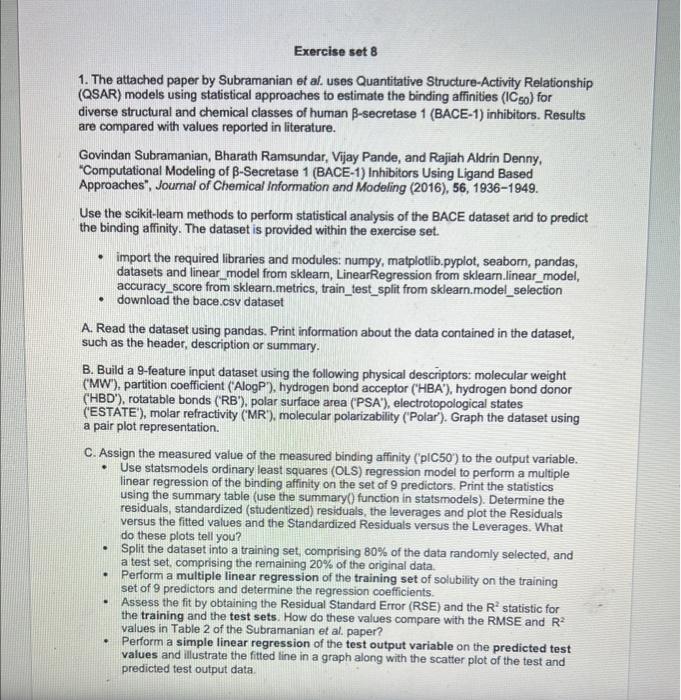

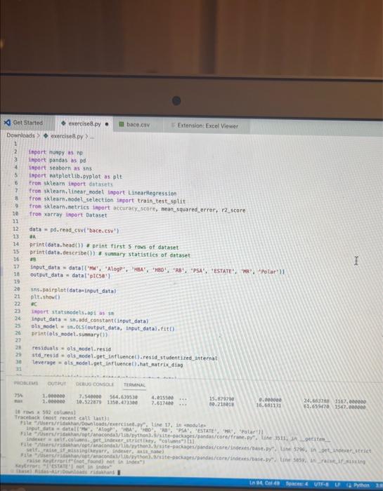
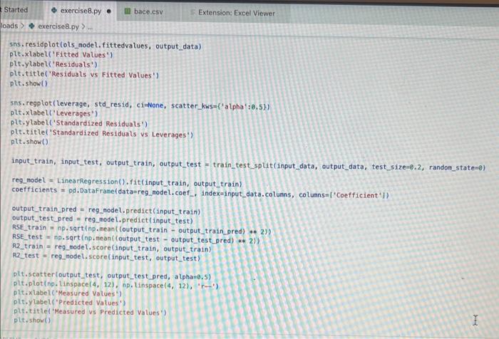
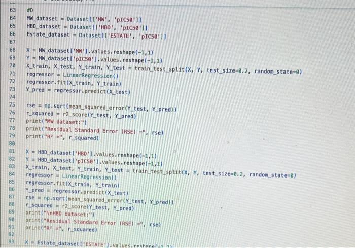
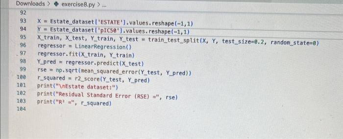Exercise set 8 1. The attached paper by Subramanian ot al. uses Quantitative Structure-Activity Relationship (QSAR) models using statistical approaches to estimate the binding affinities (C50) for diverse structural and chemical classes of human -secretase 1 (BACE-1) inhibitors. Results are compared with values reported in literature. Govindan Subramanian, Bharath Ramsundar, Vijay Pande, and Rajiah Aldrin Denny, "Computational Modeling of -Secretase 1 (BACE-1) Inhibitors Using Ligand Based Approaches", Journal of Chemical Information and Modeling (2016), 56, 1936-1949. Use the scikit-leam methods to perform statistical analysis of the BACE dataset arid to predict the binding affinity. The dataset is provided within the exercise set. - import the required libraries and modules: numpy, matplotlib.pyplot, seabom, pandas, datasets and linear_model from sklearn, LinearRegression from sklearn.linear_model, accuracy_score from sklearn.metrics, train_test_split from sklearn.model_selection - download the bace.csv dataset A. Read the dataset using pandas. Print information about the data contained in the dataset, such as the header, description or summary. B. Build a 9-feature input dataset using the following physical descriptors: molecular weight ('MW'), partition coefficient ('AlogP'), hydrogen bond acceptor ('HBA'), hydrogen bond donor ('HBD'), rotatable bonds ('RB'), polar surface area (PSA'), electrotopological states ('ESTATE'), molar refractivity ('MR'), molecular polarizability ('Polar'). Graph the dataset using a pair plot representation. C. Assign the measured value of the measured binding affinity ('plC50') to the output variable. - Use statsmodels ordinary least squares (OLS) regression model to perform a multiple linear regression of the binding affinity on the set of 9 predictors. Print the statistics using the summary table (use the summary() function in statsmodels). Determine the residuals, standardized (studentized) residuals, the leverages and plot the Residuals versus the fitted values and the Standardized Residuals versus the Leverages. What do these plots tell you? - Split the dataset into a training set, comprising 80% of the data randomly selected, and a test set, comprising the remaining 20% of the original data. - Perform a multiple linear regression of the training set of solubility on the training set of 9 predictors and determine the regression coefficients. - Assess the fit by obtaining the Residual Standard Error (RSE) and the R2 statistic for the training and the test sets. How do these values compare with the RMSE and R2 values in Table 2 of the Subramanian et al. paper? - Perform a simple linear regression of the test output variable on the predicted test values and illustrate the fitted line in a graph along with the scatter plot of the test and predicted test output data. the training and the test sets. Hew de these mives cerpare with the fuse and R2 values in Table 2 of the Subramanian of at ptpen? - Perform a simple linear rogresslan of the test output vartabie on the predicted best values and ilustrate fre filind fint in a grseh along ith the saatter plot of the test and poedicted teel outfot data. D. Conerabe an 3 single-feature dueasets by selecting only the column MrW, er HED; or 'Fstate' from the above set in pert B. - Pestont a single linear negresion on enet of the singie feature datarest usirg the approwich in part C. - How do the rests for each simgir incur ingrimen oompare with the milapie inear tegression trem purt C C? inpart nunpy as np ieport pandas as pd inpert seaboim as sns: inport natplotlib.pyplot as plt: fron sklearn inport datayets fron sklearn. Winear_nodet inport Linearflegression Irom sklearhinodelsielection inport train_test, jolit Iron sklearn, netrics laport accuracy_score, nean_squared_error, r2 score frob xarray inport Dataset data = pd. read_csv( 'bace, esy 2 r at print(data.head()) print first 5 rows of dataset print(data. detcribe()) & sumary statisties of dataset ari inpot_data = datall'Pr', 'AlogP?, 'MEAY, 'HBO', 'AE', 'PSA', 'ESTATE', 'MR', 'Aolar'll output_data = datal'ptcse'] ins+pairplot (dataninput_data) (ptt, shout) ac inport statsinodets,api as sa Input_data = st, add constant (input_data) sls_node 2= in, orsf output_data, input_data),fit() print(ots_nodel.sunary (1) residuats = ols nodel, resid std_resid o ols_nodel. get_inf luence(3, resid_stusentized internat leverage = ots_nodet,get_inftuence(), hat_matrix_diap Trarme o 592 cotiensi Tracriati (ave recent cath Lait)! raise keverrarif" (net, foumel net in Isden"). thejcriper "l Estang't net in indey- Started exercise8.py e III bace.csv Extension: Excel Viewer loads > \& exercise 8.py >.... sns. residplot (ols_nodel. fittedvalues, output_data) plt.xlabel( Fitted Values') plt.ylabel''Residuals') plt.title('Residuals vs Fitted Values') plt.show() sns. regplot (leverage, std_resid, ci=None, seatter_kws=\{'alphal: 0.5}) plt.xlabel( 'Leverages") plt.ylabel('Standardized Residuals') plt. title('standardized Residuats vs Leverages') plt.show() input_train,_input_test, output_train, output_test = train_test_sptit(input_data, output_data, test_sizeng.2, randon_state=0) req.model = LinearRegression(). fit(input_train, output_train) coefficients = pd. Dataframe(data=reg_model. coef,. index=input_data. columns, colunnsa['Coefficient']) output_train_pred = reg model.predict ( input_ t rain ) output_test_pred = reg_nodel. predict (input_test) RSE_train = np.sqrt (np.mean ( (output_train - output_train_pred) +4 21) RSE_test = np.sqrt (np.mean( (output_test - output_test_pred) kk 2)) R2 train = reg.model. score(input_train, output_train) A2 test = reg_model. score(input_test, output_test) plt.scatter(output_test, output_test_pred, atpha=0.5) plt. plot (np. tinspace (4,12),np.1 inspace(4, 12), 4r1) plt.xlabel( 'Measured Vatues') plt. ylabel( 'Predicted Vatues') plt.title( 'Measured vs Predicted Values') plt. showr) print (aR? n". r squared)