Please, I need help with this problem. Will definitely upvote!

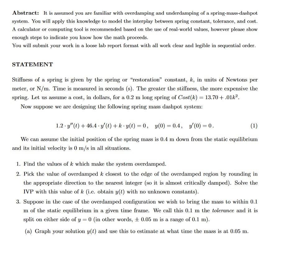
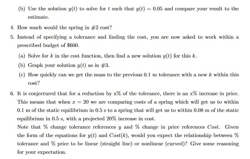
Abstract: It is assumed you are familiar with overdamping and underdamping of a spring-mass-dashpot system. You will apply this knowledge to model the interplay between spring constant, tolerance, and cost. A calculator or computing tool is recommended based on the use of real-world values, however please show enough steps to indicate you know how the math proceeds. You will submit your work in a loose lab report format with all work clear and legible in sequential order. STATEMENT Stiffness of a spring is given by the spring or restoration constant, k, in units of Newtons per meter, or N/m. Time is measured in seconds (s). The greater the stiffness, the more expensive the spring. Let us assume a cost, in dollars, for a 0.2 m long spring of Cost(k) = 13.70 +.01k2. Now suppose we are designing the following spring mass dashpot system: 1.2.y"(t) + 46.4.y'(t) +k-y(t) = 0, y(0) = 0.4, '(0)=0. (1) We can assume the initial position of the spring mass is 0.4 m down from the static equilibrium and its initial velocity is 0 m/s in all situations. 1. Find the values of k which make the system overdamped. 2. Pick the value of overdamped k closest to the edge of the overdamped region by rounding in the appropriate direction to the nearest integer (so it is almost critically damped). Solve the IVP with this value of k (i.c. obtain y(t) with no unknown constants). 3. Suppose in the case of the overdamped configuration we wish to bring the mass to within 0.1 m of the static equilibrium in a given time frame. We call this 0.1 m the tolerance and it is split on either side of y=0 (in other words, + 0.05 m is a range of 0.1 m). (a) Graph your solution y() and use this to estimate at what time the mass is at 0.05 m. (b) Use the solution y(t) to solve for t such that y(t) = 0.05 and compare your result to the estimate. 4. How much would the spring in #2 cost? 5. Instead of specifying a tolerance and finding the cost, you are now asked to work within a prescribed budget of $600. (a) Solve for k in the cost function, then find a new solution y(t) for this k. (b) Graph your solution y(t) as in #3. (c) How quickly can we get the mass to the previous 0.1 m tolerance with a new k within this cost? 6. It is conjectured that for a reduction by x% of the tolerance, there is an x% increase in price. This means that when I = 20 we are comparing costs of a spring which will get us to within 0.1 m of the static equilibrium in 0.5 s to a spring that will get us to within 0.08 m of the static equilibrium in 0.5 s, with a projected 20% increase in cost. Note that % change tolerance references y and % change in price references Cost. Given the form of the equations for y(t) and Cost(k), would you expect the relationship between % tolerance and % price to be linear (straight line) or nonlinear (curved)? Give some reasoning for your expectation. Abstract: It is assumed you are familiar with overdamping and underdamping of a spring-mass-dashpot system. You will apply this knowledge to model the interplay between spring constant, tolerance, and cost. A calculator or computing tool is recommended based on the use of real-world values, however please show enough steps to indicate you know how the math proceeds. You will submit your work in a loose lab report format with all work clear and legible in sequential order. STATEMENT Stiffness of a spring is given by the spring or restoration constant, k, in units of Newtons per meter, or N/m. Time is measured in seconds (s). The greater the stiffness, the more expensive the spring. Let us assume a cost, in dollars, for a 0.2 m long spring of Cost(k) = 13.70 +.01k2. Now suppose we are designing the following spring mass dashpot system: 1.2.y"(t) + 46.4.y'(t) +k-y(t) = 0, y(0) = 0.4, '(0)=0. (1) We can assume the initial position of the spring mass is 0.4 m down from the static equilibrium and its initial velocity is 0 m/s in all situations. 1. Find the values of k which make the system overdamped. 2. Pick the value of overdamped k closest to the edge of the overdamped region by rounding in the appropriate direction to the nearest integer (so it is almost critically damped). Solve the IVP with this value of k (i.c. obtain y(t) with no unknown constants). 3. Suppose in the case of the overdamped configuration we wish to bring the mass to within 0.1 m of the static equilibrium in a given time frame. We call this 0.1 m the tolerance and it is split on either side of y=0 (in other words, + 0.05 m is a range of 0.1 m). (a) Graph your solution y() and use this to estimate at what time the mass is at 0.05 m. (b) Use the solution y(t) to solve for t such that y(t) = 0.05 and compare your result to the estimate. 4. How much would the spring in #2 cost? 5. Instead of specifying a tolerance and finding the cost, you are now asked to work within a prescribed budget of $600. (a) Solve for k in the cost function, then find a new solution y(t) for this k. (b) Graph your solution y(t) as in #3. (c) How quickly can we get the mass to the previous 0.1 m tolerance with a new k within this cost? 6. It is conjectured that for a reduction by x% of the tolerance, there is an x% increase in price. This means that when I = 20 we are comparing costs of a spring which will get us to within 0.1 m of the static equilibrium in 0.5 s to a spring that will get us to within 0.08 m of the static equilibrium in 0.5 s, with a projected 20% increase in cost. Note that % change tolerance references y and % change in price references Cost. Given the form of the equations for y(t) and Cost(k), would you expect the relationship between % tolerance and % price to be linear (straight line) or nonlinear (curved)? Give some reasoning for your expectation