

Answered step by step
Verified Expert Solution
Question
1 Approved Answer
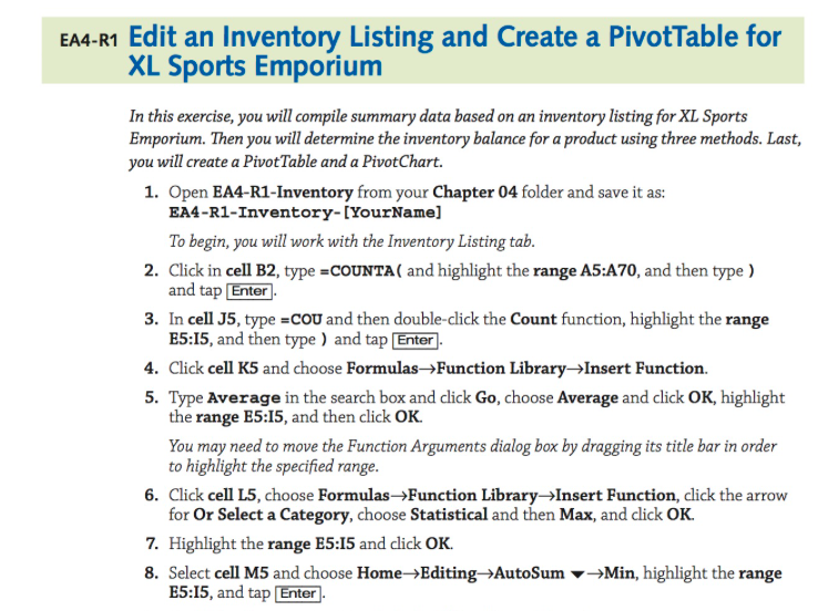
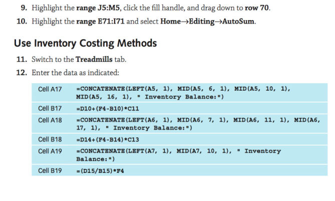
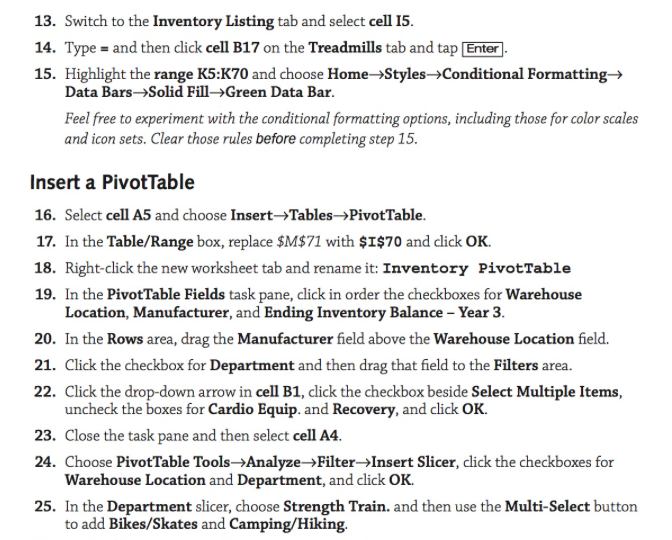
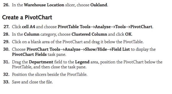
PLEASE MAKE SURE YOU DO A EXCEL FORMAT SCREEN SHOT OR WRITE IT OR ANY OTHER FORMAT THAT SHOWS THE WORK!!!!!!!!!! EA4-R1 Edit an Inventory
 PLEASE MAKE SURE YOU DO A EXCEL FORMAT SCREEN SHOT OR WRITE IT OR ANY OTHER FORMAT THAT SHOWS THE WORK!!!!!!!!!!
Step by Step Solution
There are 3 Steps involved in it
Step: 1

Get Instant Access to Expert-Tailored Solutions
See step-by-step solutions with expert insights and AI powered tools for academic success
Step: 2

Step: 3
Ace Your Homework with AI
Get the answers you need in no time with our AI-driven, step-by-step assistance
Get Started
New Trends In Databases And Information Systems ADBIS 2015 Short Papers And Workshops BigDap DCSA GID MEBIS OAIS SW4CH WISARD Poitiers In Computer And Information Science 539
Authors: Tadeusz Morzy ,Patrick Valduriez ,Ladjel Bellatreche
1st Edition
3319232002, 978-3319232003