Please provide compelte solution, show full calculations, explanations and proofs to the following question:

Please only answer question 2 only

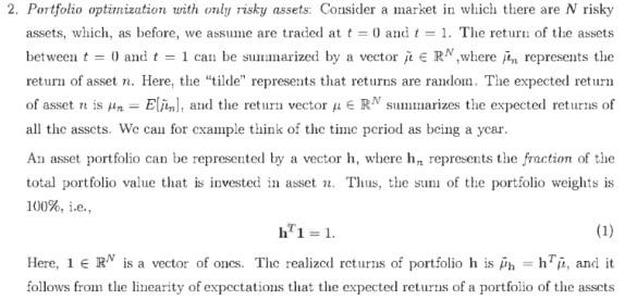
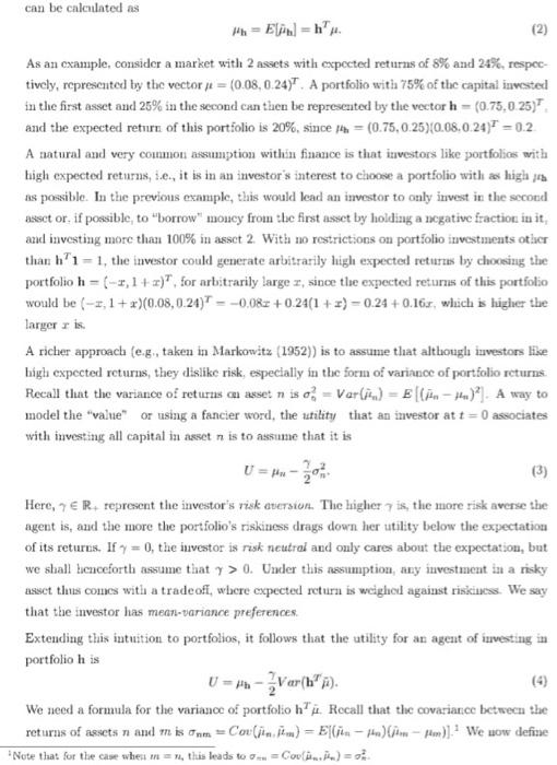
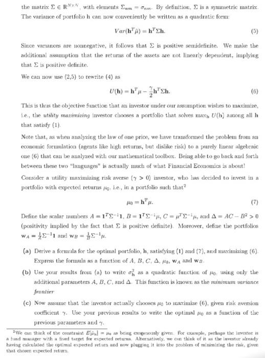
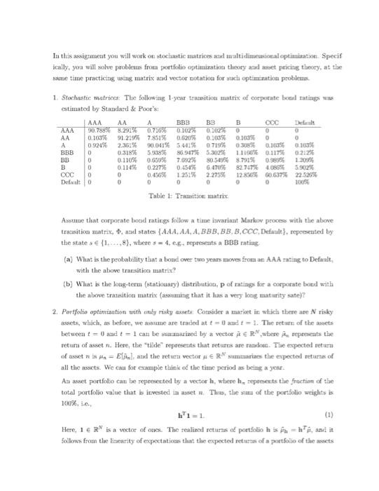
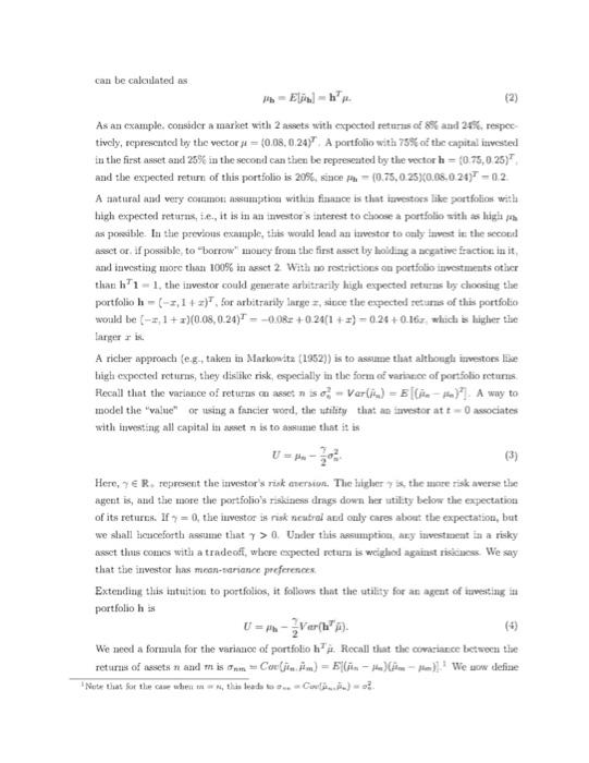
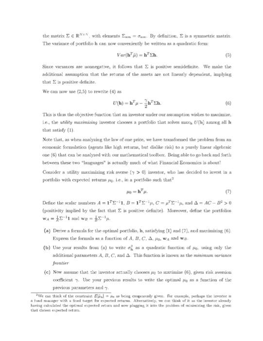
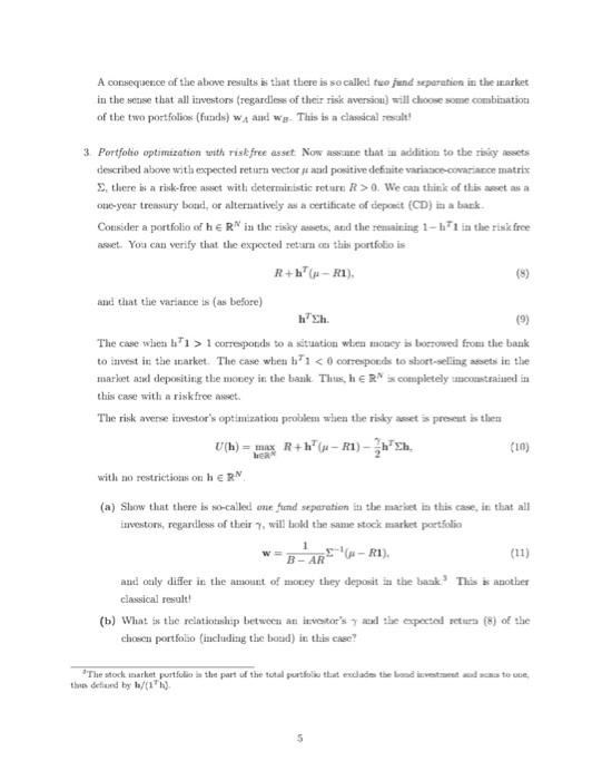
2. Portfolio optimization with only risky assets: Consider a market in which there are N risky assets, which, as before, we assume are traded at t = 0 and t = 1. The return of the assets between t = 0 and t = 1 can be summarized by a vector i E RN where in represents the return of asset n. Here, the "tilde" represents that returns are random. The expected return of asset it is An = Elind, and the return vector HE RN summarizes the expected returns of all the assets. We can for example think of the time period as being a year. An asset portfolio can be represented by a vector h, where he represents the fraction of the total portfolio value that is invested in asset . Thus, the sum of the portfolio weights is 100%. i.e., h"1=1. (1) Here, 1 E R is a vector of ones. The realized returns of portfolio h is in = hit, and it follows from the linearity of expectations that the expected returns of a portfolio of the assets can be calculated as El = h' (2) As an example, consider a market with 2 assets with expected returns of 8% and 24%, respec tively, represented by the vector de = (0.08, 0.24) A portfolio with 75% of the capital invested in the first asset and 25% in the second can then be represented by the vector h = (0.75,0.25) and the expected return of this portfolio is 20%, since it = (0.75, 0.25)(0.08.0.24)" = 0.2 A natural and very common assumption within finance is that investors like portfolios with high expected returns, i.e., it is in an investor's interest to choose a portfolio with a high as possible. In the previous example, this would lead an investor to only invest in the second assct or if possible to borrow" moncy from the first asset by holding a negative fraction in it, and investing more than 100% in asset 2 With no restrictions on portfolio investments otser thanh' 1 - 1, the investor could generate arbitrarily high expected returres by choosing the portfolio h = (-1, 1+x)". for arbitrarily large I, since the expected returns of this portfolio would be (-1,1 + x)(0.08,0.24) * = -0,082 +0.24(1 + 2) = 0.24 +0.16r, which is higher the larger ris. A richer approach (e.g., taken in Markowitz (1952)) is to assume that although izvestors like high expected returns they dislike risk, especially in the form of varianoe of portfolio returns. Recall that the variance of returns classet niso - Var() - (An - Hu)?). A way to model the value or tising a fancier word, the utility that an investor at t=0 associates with investing all capital in asset n is to assume that it is (3) Here, 7 R. represent the investor's risk version. The higher is, the more risk averse the agent is, and the more the portfolio's riskiness drags down her utility below the expectation of its retures. If y = 0, the investor is risk neutral and only cares about the expectation, but we shall licnceforth assume that y > 0. Under this assumption, any investment in a risky assct this comes with a tradeoff, were expected return is weighed against riskuess. We say that the investor has mean-variance preferences Extending this intuition to portfolios, it follows that the utility for an agent of investing in portfolio his U = "-Var(h"). We need a formula for the variance of portfolio h". Rocall that the covariance between the returns of assets n and mis onm = Covljite n) = E|--H)].? We now define Note that for the case wher, this leads to it. Col.) the matrix SERVx, with clements Com By definition, is a symmetric matrix The variance of portfolio h can now conveniently be written as a quadratic form: Var(h") = heh. (5) Since variances are nonnegative, it follows that is positive senidetinite. We make the additional assumption that the returns of the assets are not linearly dependent, implying that is positive definite. We can now use (2,5) to rewrite (4) as (6) This is thus the objective function that an investor under our assumption wishes to maximize, ie, the utility maximizing investor chooses a portfolio that solves max. (h) among all h that satisfy (1) Note that, as when analyzing the law of one price, we have transformed the problem from an economic forumlation (agents like light returns, but dislike risk) to a purely linear algebraic oue (6) that can be analyzed with our mathematical toolbox. Being able to go back and forth between these two "languages" is actually much of what Financial Economics is about! Consider a utility maximizing risk averse (> 0) investor, who has decided to invest in a portfolio with expected returns tule, in a portfolio such that? (7) Define the scalar mmbers A = 175-1, B=175+ C = "--, and A = AC-B2 > 0 (positivity implied by the fact that is positive definite). Moreover, vefine the portfolios WA = 481 and we = . (a) Derive a formula for the optimal portfolio, h, satisfying (1) and (7), and maximizing (6) Express the formula as a function of A, B, C, A, HO WA and we (b) Use your results from (a) to write of as a quadratic function of Housing only the additional parameters A, B, C, and A This function is known as the minimum wariance frontier (c) Now assume that the investor actually chooses to to watimize (6), given risk aversion coefficient 7. Use your previous results to write the optimal Ho as a function of thic previous parameters and * We can think of the constraint EwHo as being coasty given For example, perhaps the investotis a fund nuper with a fixed target for expected returns Alternatively, we can think of it as the investur already having calculated the optimal expected return and now plugging it into the problem of minimizing the risk given that chosen expected retum. A consequence of the above results is that there is so called two fund separation in the inarket in the sense that all investors (regardless of their risk aversion) will choose some combination of the two portfolios (funds) wA and wg. This is a classical result! In this assignment you will work on stochastic matrices al multidimensional optimization Specif Senlly, you will solve problemus from portfolio optimization theory and reset pracing theory, at the same time practicing wing matrix atud vector notation for such optimization probleme 1. Stochastic matrices. The following 1-year transitioti mattix of corporate botul tating was estimated by Standard & Poor's AAA BBB BB B Det AAA 90.783% 8,291% 0.726% 0.102 0.102% 0 0 AA 0.1038 91.219% 7.851% 0.6205 0.100% 0.1005 0 0 0.924% 2.36% 30.041% 5.411% 0719% 03085 0.100 01635 BBB 0.3185 5.9% 86.947% 5.3027 1110 0111 0212 BB 0 0.110% 0:659% 7.092% 80509% 8.7915 1.2004 B 0 0.1145 0.227% 0.454% G470% 82.707540865 5902% 0.156% 1.251 2.275% 12836 0.637% 22.5265 Defit 0 0 0 0 0 A 0 0 0 0 Table 1 Transitio matrix Asstime that corporate bond ratings follow a time iwariant Markow process with the above transition matrix, and states (AAA, AA, A, BBB, BB,B,CCC Default), represented by the state 1...,8), where s= 1. es represents a BBB rating (a) What is the probability that a bond over two years moes from a AAA rating to Default with the above transition matrix? (b) What is the long-term (stationary) distributit, pof ratings for a corporate bond with the above transition matrix (assuming that it lus a very long maturity sate)? 2. Portfolio optimization with enty risky asseta Consider a market in stich there are N risky assets, which is before, we assume are traded at t = 0 and t = 1. The reture of the assets between t = 0 and t = 1 cats be sumarized by a vector is Rwhere represents the return of asset n. Here, the "tilde represents that returns are randon. The expected return of asset til din = Elful, and the return vector sumusuarides the expected returns of all the asscts. We cau for example think of the time period as being a year. An asset portfolio can be represented to a vector h, where he represents the fraction of the total portfolio value that is invested in asset . Thies, the sana of the portfolio weights is 100%. (1) Here, 1 E R is a vector of ones. The realized returns of portfolio his-hi, and it follows from the liscarity of exportationes that the expected returres of a portfolio of the assets can be calculated as -El- (2) As an example, consider a market with 2 assets with expected returns of 85 and 24%, respec tively, represented by the vector pe=0.08, 0.247" A portfolio wit 75% of the capital invested in the first asset and 25% in the second can then be represented by the vector h= (0.75, 0.25) and the expected return of this portfolio is 20%, since A - (0.75, 0.2530.08.0.24)" - 02. A natural and very counts assumption within finance is that ivestors like portfolios with high expected returns, ie, it is in an investors interest to choose a portfolio sith as as higlar les poesibile. In the previous example, this world lead an tovestor to only invest in the second aset or if possible to borrow" money from the first asset by holding a negative fraction in it, and investing more than 100% in assct 2 With no restrictions on portfolio investments other that h1 - 1, the investor could generate arisitrarily high expected returns by choosing the portfolio h = (-3,1 + 2)", for arbitrarily largez, since the expected returns of this portfolio wenuld be (-=, 1+2)(0.08, 0.24)" = -0.082 +0.24[1 + 1) = 0.24 +0.163 which is higher the larger ris. A richer approach (eg, taken in Markowita (1952)) is to assume that although investors like high expected returns, they dislike risk, especially in the form o varie of portfolio retams Recall that the variance of returus can asset no-Varliu) = [(-)! A way to model the "wale" or using a fancier word, the utility that an westor att associates with investing all capital in wet n is to assume that it is Here, 7 Rrepresent the investor's risk ezersion. The higher 7 the mare zisk averse the agent is, and the more the portfolio's riskiness drags down her utility below the expectation of its retures. If = 0, the investor is risk neutral and caly cares about the expectation, but we shall cuceforth assume that > 0. Under this assumption, any investuat in a risky arset thues comunes with a tradeofi, wbore expected return is weighed against risic We say that the investor has mean-tariance preferencer Extending this intuition to portfolios, it follows that the utility for an agent of survesting in portfolio his We need a formula for the variance of portfolio bi. Rocall that the covariance between the returns of assets n and mis on = Core(jta. m) = Ellin - 3)(from Hem). We now define Note that for the case whetti within a Cel.)? the matrix LERN* with elements En By definition. I is a symmetric matrix The variance of portfolo h can now conveniently be written as a quadratic forms: Varih")=bh Since variances are sounegative, it follows that is positive senidefinite We make the additional assumption that the returns of the assets are not linearly dependent, implying that is positive definite We can now use (2,5) to rewrite (4) as (6) This is thus the objective function that at trestoruder our assumption wishes to uscitize. Le, the wtlity maximizing investor chooses a portfolio that solves me U/h) among all h that satisfy (1) Note that, as when analyzing the law of one price, we have transformed the problem from an economic Forumintios (agents like Irigt returns, but dislike task) to a purely fiteat algelenie one (6) that can be annlyzed with our mathematical toolbox. Being able to go back and forth between these two "languages" is actually much of what Financial Economies is about! Consider a utility maximizing risk avere (o > 0) investor, who was decided to invest in a portfolio with expected returns pole, in a portfolio such that? H = h. Define the scalar mumbers A 175-1. B = 12-CEE, and A - AC - 320 (positivity implied by the fact that is positive definite). Moreover, define the portfolio WA-1-1 and was (a) Derive a formula for the optimal portfolio, h, satisfying (1) and (7), and maximizing (6) Express the formula as a function of A, B, C, A., WA and we (b) Use your results from (a) to write as a quadratic function of poing only the aditional parameters A, B, C, and A This function is not as the minimum tariance frontier (c) Now assume that the investor actually choses po to saximize (6) gives rise avesion coefficient. Use your previous results to write the optimal 4 as a function of the previous parameters and We can think of the construit Amberg only en Pue ample, the the last tander with ford target for expected Alternatively, we think of the lady having calculated the optimal expected to and plugging it into the publiciting the risk givet A consequence of the above results is that there is so called two jund separation in the market in the sense that all investors (regardless of their risk aversion) will choose some combination of the two portfolios (funds) wAand wg. This is a classical result 3 Portfolio optimization with risk-free asset Now assue that an addition to the riskynsets described above with expected return vector je nad positive definite variatico.cariance matrix Ethere it a risk-froe nect with deterministic retur R > 0. We can think of this aset as a one-year trentury brand, or alternatively as a certificate of deposit (CD) in a bank Consider a portfolio of her in the risky anets, and the remaining 1-b1 in the risk free asset. You can verify that the expected return co this portfolio is R+"-RI). (5) and that the variance is (as before) (9) The case wlicni b'1 > 1 corresponds to a situation when money is borrowed from the bank to invest in the market. The case when t'i 0. Under this assumption, any investment in a risky assct this comes with a tradeoff, were expected return is weighed against riskuess. We say that the investor has mean-variance preferences Extending this intuition to portfolios, it follows that the utility for an agent of investing in portfolio his U = "-Var(h"). We need a formula for the variance of portfolio h". Rocall that the covariance between the returns of assets n and mis onm = Covljite n) = E|--H)].? We now define Note that for the case wher, this leads to it. Col.) the matrix SERVx, with clements Com By definition, is a symmetric matrix The variance of portfolio h can now conveniently be written as a quadratic form: Var(h") = heh. (5) Since variances are nonnegative, it follows that is positive senidetinite. We make the additional assumption that the returns of the assets are not linearly dependent, implying that is positive definite. We can now use (2,5) to rewrite (4) as (6) This is thus the objective function that an investor under our assumption wishes to maximize, ie, the utility maximizing investor chooses a portfolio that solves max. (h) among all h that satisfy (1) Note that, as when analyzing the law of one price, we have transformed the problem from an economic forumlation (agents like light returns, but dislike risk) to a purely linear algebraic oue (6) that can be analyzed with our mathematical toolbox. Being able to go back and forth between these two "languages" is actually much of what Financial Economics is about! Consider a utility maximizing risk averse (> 0) investor, who has decided to invest in a portfolio with expected returns tule, in a portfolio such that? (7) Define the scalar mmbers A = 175-1, B=175+ C = "--, and A = AC-B2 > 0 (positivity implied by the fact that is positive definite). Moreover, vefine the portfolios WA = 481 and we = . (a) Derive a formula for the optimal portfolio, h, satisfying (1) and (7), and maximizing (6) Express the formula as a function of A, B, C, A, HO WA and we (b) Use your results from (a) to write of as a quadratic function of Housing only the additional parameters A, B, C, and A This function is known as the minimum wariance frontier (c) Now assume that the investor actually chooses to to watimize (6), given risk aversion coefficient 7. Use your previous results to write the optimal Ho as a function of thic previous parameters and * We can think of the constraint EwHo as being coasty given For example, perhaps the investotis a fund nuper with a fixed target for expected returns Alternatively, we can think of it as the investur already having calculated the optimal expected return and now plugging it into the problem of minimizing the risk given that chosen expected retum. A consequence of the above results is that there is so called two fund separation in the inarket in the sense that all investors (regardless of their risk aversion) will choose some combination of the two portfolios (funds) wA and wg. This is a classical result! In this assignment you will work on stochastic matrices al multidimensional optimization Specif Senlly, you will solve problemus from portfolio optimization theory and reset pracing theory, at the same time practicing wing matrix atud vector notation for such optimization probleme 1. Stochastic matrices. The following 1-year transitioti mattix of corporate botul tating was estimated by Standard & Poor's AAA BBB BB B Det AAA 90.783% 8,291% 0.726% 0.102 0.102% 0 0 AA 0.1038 91.219% 7.851% 0.6205 0.100% 0.1005 0 0 0.924% 2.36% 30.041% 5.411% 0719% 03085 0.100 01635 BBB 0.3185 5.9% 86.947% 5.3027 1110 0111 0212 BB 0 0.110% 0:659% 7.092% 80509% 8.7915 1.2004 B 0 0.1145 0.227% 0.454% G470% 82.707540865 5902% 0.156% 1.251 2.275% 12836 0.637% 22.5265 Defit 0 0 0 0 0 A 0 0 0 0 Table 1 Transitio matrix Asstime that corporate bond ratings follow a time iwariant Markow process with the above transition matrix, and states (AAA, AA, A, BBB, BB,B,CCC Default), represented by the state 1...,8), where s= 1. es represents a BBB rating (a) What is the probability that a bond over two years moes from a AAA rating to Default with the above transition matrix? (b) What is the long-term (stationary) distributit, pof ratings for a corporate bond with the above transition matrix (assuming that it lus a very long maturity sate)? 2. Portfolio optimization with enty risky asseta Consider a market in stich there are N risky assets, which is before, we assume are traded at t = 0 and t = 1. The reture of the assets between t = 0 and t = 1 cats be sumarized by a vector is Rwhere represents the return of asset n. Here, the "tilde represents that returns are randon. The expected return of asset til din = Elful, and the return vector sumusuarides the expected returns of all the asscts. We cau for example think of the time period as being a year. An asset portfolio can be represented to a vector h, where he represents the fraction of the total portfolio value that is invested in asset . Thies, the sana of the portfolio weights is 100%. (1) Here, 1 E R is a vector of ones. The realized returns of portfolio his-hi, and it follows from the liscarity of exportationes that the expected returres of a portfolio of the assets can be calculated as -El- (2) As an example, consider a market with 2 assets with expected returns of 85 and 24%, respec tively, represented by the vector pe=0.08, 0.247" A portfolio wit 75% of the capital invested in the first asset and 25% in the second can then be represented by the vector h= (0.75, 0.25) and the expected return of this portfolio is 20%, since A - (0.75, 0.2530.08.0.24)" - 02. A natural and very counts assumption within finance is that ivestors like portfolios with high expected returns, ie, it is in an investors interest to choose a portfolio sith as as higlar les poesibile. In the previous example, this world lead an tovestor to only invest in the second aset or if possible to borrow" money from the first asset by holding a negative fraction in it, and investing more than 100% in assct 2 With no restrictions on portfolio investments other that h1 - 1, the investor could generate arisitrarily high expected returns by choosing the portfolio h = (-3,1 + 2)", for arbitrarily largez, since the expected returns of this portfolio wenuld be (-=, 1+2)(0.08, 0.24)" = -0.082 +0.24[1 + 1) = 0.24 +0.163 which is higher the larger ris. A richer approach (eg, taken in Markowita (1952)) is to assume that although investors like high expected returns, they dislike risk, especially in the form o varie of portfolio retams Recall that the variance of returus can asset no-Varliu) = [(-)! A way to model the "wale" or using a fancier word, the utility that an westor att associates with investing all capital in wet n is to assume that it is Here, 7 Rrepresent the investor's risk ezersion. The higher 7 the mare zisk averse the agent is, and the more the portfolio's riskiness drags down her utility below the expectation of its retures. If = 0, the investor is risk neutral and caly cares about the expectation, but we shall cuceforth assume that > 0. Under this assumption, any investuat in a risky arset thues comunes with a tradeofi, wbore expected return is weighed against risic We say that the investor has mean-tariance preferencer Extending this intuition to portfolios, it follows that the utility for an agent of survesting in portfolio his We need a formula for the variance of portfolio bi. Rocall that the covariance between the returns of assets n and mis on = Core(jta. m) = Ellin - 3)(from Hem). We now define Note that for the case whetti within a Cel.)? the matrix LERN* with elements En By definition. I is a symmetric matrix The variance of portfolo h can now conveniently be written as a quadratic forms: Varih")=bh Since variances are sounegative, it follows that is positive senidefinite We make the additional assumption that the returns of the assets are not linearly dependent, implying that is positive definite We can now use (2,5) to rewrite (4) as (6) This is thus the objective function that at trestoruder our assumption wishes to uscitize. Le, the wtlity maximizing investor chooses a portfolio that solves me U/h) among all h that satisfy (1) Note that, as when analyzing the law of one price, we have transformed the problem from an economic Forumintios (agents like Irigt returns, but dislike task) to a purely fiteat algelenie one (6) that can be annlyzed with our mathematical toolbox. Being able to go back and forth between these two "languages" is actually much of what Financial Economies is about! Consider a utility maximizing risk avere (o > 0) investor, who was decided to invest in a portfolio with expected returns pole, in a portfolio such that? H = h. Define the scalar mumbers A 175-1. B = 12-CEE, and A - AC - 320 (positivity implied by the fact that is positive definite). Moreover, define the portfolio WA-1-1 and was (a) Derive a formula for the optimal portfolio, h, satisfying (1) and (7), and maximizing (6) Express the formula as a function of A, B, C, A., WA and we (b) Use your results from (a) to write as a quadratic function of poing only the aditional parameters A, B, C, and A This function is not as the minimum tariance frontier (c) Now assume that the investor actually choses po to saximize (6) gives rise avesion coefficient. Use your previous results to write the optimal 4 as a function of the previous parameters and We can think of the construit Amberg only en Pue ample, the the last tander with ford target for expected Alternatively, we think of the lady having calculated the optimal expected to and plugging it into the publiciting the risk givet A consequence of the above results is that there is so called two jund separation in the market in the sense that all investors (regardless of their risk aversion) will choose some combination of the two portfolios (funds) wAand wg. This is a classical result 3 Portfolio optimization with risk-free asset Now assue that an addition to the riskynsets described above with expected return vector je nad positive definite variatico.cariance matrix Ethere it a risk-froe nect with deterministic retur R > 0. We can think of this aset as a one-year trentury brand, or alternatively as a certificate of deposit (CD) in a bank Consider a portfolio of her in the risky anets, and the remaining 1-b1 in the risk free asset. You can verify that the expected return co this portfolio is R+"-RI). (5) and that the variance is (as before) (9) The case wlicni b'1 > 1 corresponds to a situation when money is borrowed from the bank to invest in the market. The case when t'i