please solve for analysis - everything is provided below

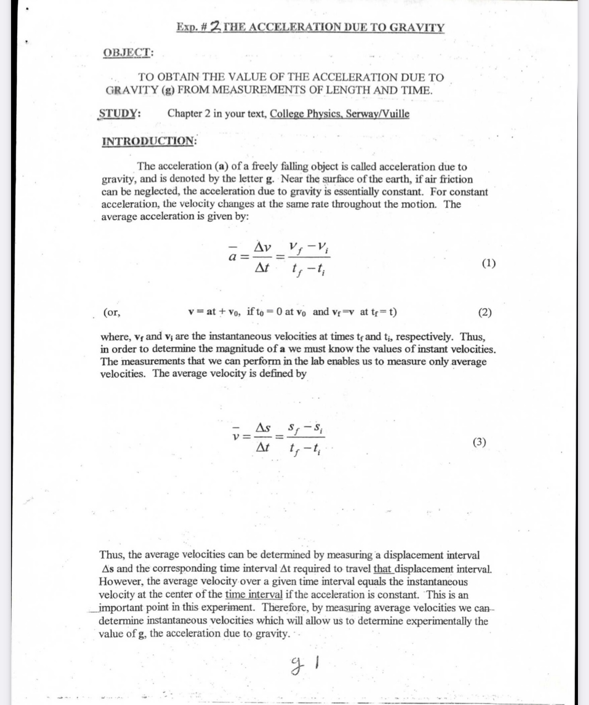
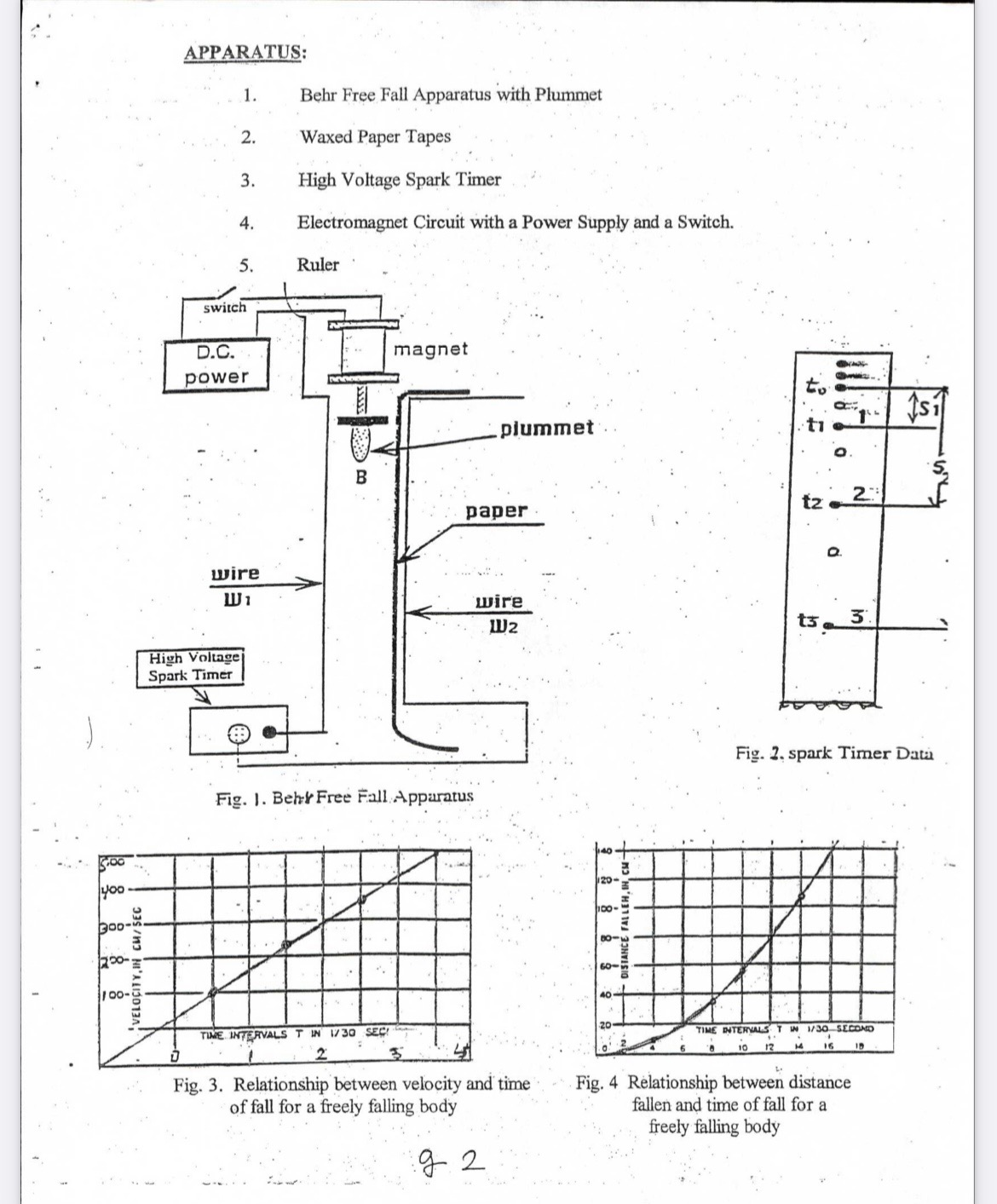
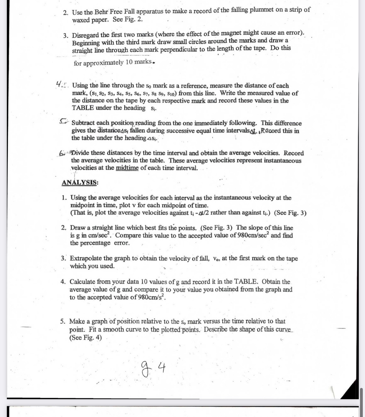
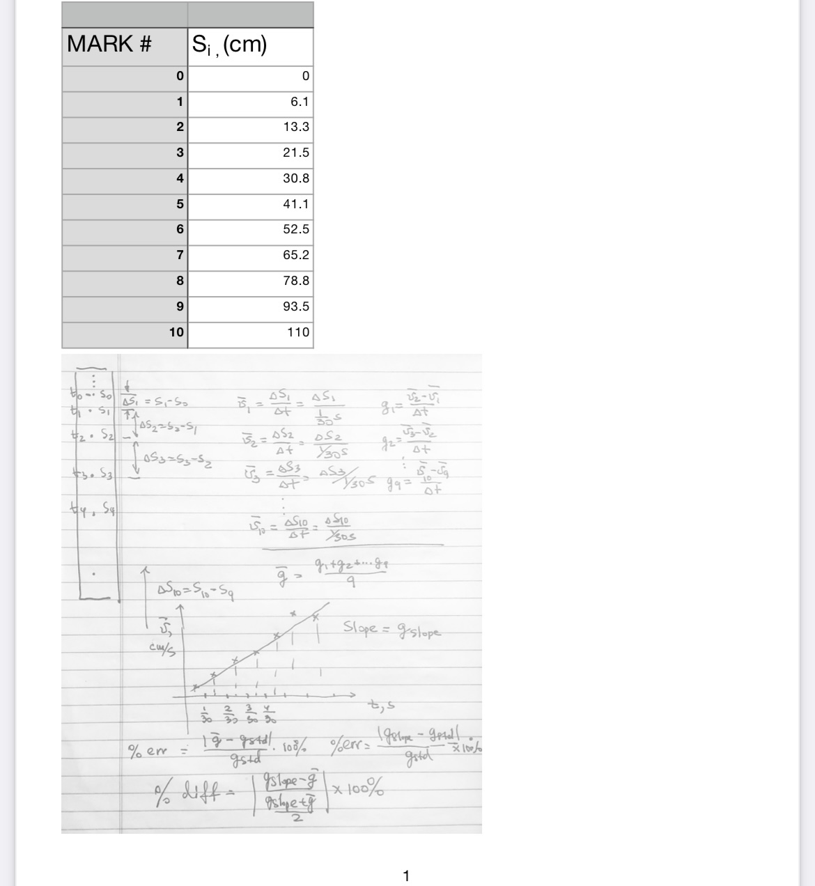
Exp. # 2 THE ACCELERATION DUE TO GRAVITY OBJECT: TO OBTAIN THE VALUE OF THE ACCELERATION DUE TO GRAVITY (g) FROM MEASUREMENTS OF LENGTH AND TIME. STUDY: Chapter 2 in your text, College Physics, Serway/Vuille INTRODUCTION: The acceleration (a) of a freely falling object is called acceleration due to gravity, and is denoted by the letter g. Near the surface of the earth, if air friction can be neglected, the acceleration due to gravity is essentially constant. For constant acceleration, the velocity changes at the same rate throughout the motion. The average acceleration is given by: Av V a = At (1) (or, v = at + vo, ifto = 0 at vo and vr=v at t;= t) (2) where, vr and v; are the instantaneous velocities at times ty and ti, respectively. Thus, in order to determine the magnitude of a we must know the values of instant velocities. The measurements that we can perform in the lab enables us to measure only average velocities. The average velocity is defined by AS S At -t (3) Thus, the average velocities can be determined by measuring a displacement interval As and the corresponding time interval At required to travel that displacement interval. However, the average velocity over a given time interval equals the instantaneous velocity at the center of the time interval if the acceleration is constant. This is an important point in this experiment. Therefore, by measuring average velocities we can- determine instantaneous velocities which will allow us to determine experimentally the value of g, the acceleration due to gravity. . 2 1APPARATUS: 1. Behr Free Fall Apparatus with Plummet 2. Waxed Paper Tapes 3. High Voltage Spark Timer 4. Electromagnet Circuit with a Power Supply and a Switch. 5. Ruler switch D.C. magnet power plummet . B paper wire W 1 wire 3 W2 High Voltage Spark Timer Fig. 2. spark Timer Data Fig. 1. Behr Free Fall Apparatus you BOD VELOCITY, IN CM/ SEC 100-5 TIME INTERVALS T IN 1/ 30 SEC Fig. 3. Relationship between velocity and time Fig. 4 Relationship between distance of fall for a freely falling body fallen and time of fall for a freely falling body 9 22. Use the Behr Free Fall apparatus to make a record of the falling plummet on a strip of waxed paper. See Fig. 2. 3. Disregard the first two marks (where the effect of the magnet might cause an error). Beginning with the third mark draw small circles around the marks and draw a straight line through each mark perpendicular to the length of the tape. Do this for approximately 10 marks. 4.". Using the line through the so mark as a reference, measure the distance of each mark, ($1, $2, $3, $4, $5, $6, $7, $8 59, $10) from this line. Write the measured value of the distance on the tape by each respective mark and record these values in the TABLE under the heading Si- Subtract each position reading from the one immediately following. This difference gives the distanceds; fallen during successive equal time intervalsAt Record this in the table under the heading ASi- 6Divide these distances by the time interval and obtain the average velocities. Record the average velocities in the table. These average velocities represent instantaneous velocities at the midtime of each time interval. . . ANALYSIS: 1. Using the average velocities for each interval as the instantaneous velocity at the midpoint in time, plot v for each midpoint of time. (That is, plot the average velocities against t; - 4t/2 rather than against ti.) (See Fig. 3) 2. Draw a straight line which best fits the points. (See Fig. 3) The slope of this line is g in cm/sec . Compare this value to the accepted value of 980cm/sec and find the percentage error. 3. Extrapolate the graph to obtain the velocity of fall, vo, at the first mark on the tape which you used. 4. Calculate from your data 10 values of g and record it in the TABLE. Obtain the average value of g and compare it to your value you obtained from the graph and to the accepted value of 980cm/s'. 5. Make a graph of position relative to the s. mark versus the time relative to that point. Fit a smooth curve to the plotted points. Describe the shape of this curve (See Fig. 4)MARK # Si (cm) 0 0 6.1 N d 13.3 21.5 4 30.8 41.1 6 52.5 65.2 78.8 CO 93.5 10 110 to -. So ASI = SI -SO #2 . 5 2 185 2 25 2- S At 15 2 = 052 DS2 At $3 . 53 gg= 10 of ySos AS10 = Spo - Sq 9 Slope = g slope 30 30 30 Do -. 10/ of err= 198top - getall 95+d - X 109/ of diff - 9slope - 8 X 100 /