please solve it in MATHLAB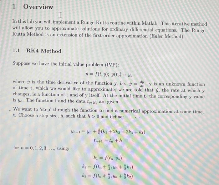

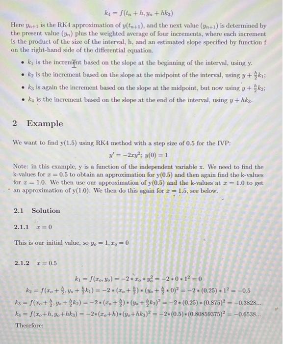
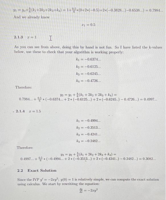
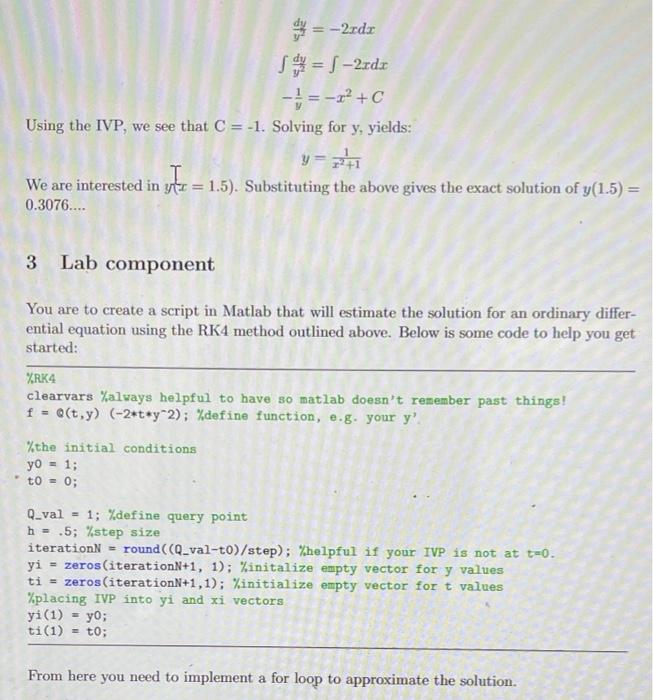
1 Overview I In this lab you will implement a Runge-Kutta routine within Matlab. This iterative method will allow you to approximate solutions for ordinary differential equations. The Runge- Kutta Method is an extension of the first-order approximation (Euler Method). 1.1 RK4 Method Suppose we have the initial value problem (IVP): = f(t,y); y(to) = yo where y is the time derivative of the function y, i.e. = y is an unknown function of time t, which we would like to approximate; we are told that y, the rate at which y changes, is a function of t and of y itself. At the initial time to the corresponding y value is yo. The function f and the data to, yo are given. We want to 'step' through the function to find a numerical approximation at some time, t. Choose a step size, h, such that h> 0 and define: Yn+1 = yn + (k+ 2ky + 2k3 + ka) In+1 = tn +h for n = 0,1,2,3,..., using: k = f(tn, yn) ky = f(tn +, Yn+ki) k3 = f(tr+ , yn + ku) ka = f(t. + h, yn + hky) Here Yn+1 is the RK4 approximation of y(tu+1), and the next value (yn+1) is determined by the present value (9) plus the weighted average of four increments, where each increment is the product of the size of the interval, h, and an estimated slope specified by function f on the right-hand side of the differential equation. ky is the increment based on the slope at the beginning of the interval, using y. ky is the increment based on the slope at the midpoint of the interval, using y + ki; ky is again the increment based on the slope at the midpoint, but now using y + $k2; ks is the increment based on the slope at the end of the interval, using y + hkz. 2 Example We want to find y(1.5) using RK4 method with a step size of 0.5 for the IVP: y = -2ry': y(0) = 1 Note: in this example, y is a function of the independent variable x. We need to find the k-values for r=0.5 to obtain an approximation for y(0.5) and then again find the k-values for 1 = 1.0. We then use our approximation of y(0.5) and the k-values at r = 1.0 to get an approximation of y(1.0). We then do this again for I = 1.5. see below. a 2.1 Solution 2.1.1 =0 This is our initial value, so yo = 1,1 = 0 2.1.2 I=0.5 k = f(x,y) = -2*1.*y=-2.0.12 = 0 ky = f(*.+5:40 + $ky)= -2+(10+)*(30++0)= -2. (0,25) + 12 = -0.5 ks = $(to +5,90 + $k2) = -2.(4.+ ). (%+ $ka) = -2* (0.25) + (0.875)2 = -0.382.... ka = $(to+h, ye+hkg) = -2.(Fo+h)-(%.+hky)2 = -2.(0.5) - (0.80859375)2 = -0.6538... Therefore: n1 = y.+ (ki+2ky+2k3+ka) = 1+ *** (0+2+(-0.5)+2+(-0.382...) -0.653...) = 0.7984... And we already knew 31 = 0,5 2.1.3 = 1 I As you can see from above, doing this by hand is not fun. So I have listed the k-values below, use these to check that your algorithm is working properly: ki = -0.6374... 12 = -0.6125... k3 = -0.6245... ke = -0.4726... Therefore 32 = 3/1 + $(+2k2 + 2ks + ka) = 0.7984... + 3+ (-0.6374... +2+(-0.6125 ...) +2+(-0.6245..) - 0.4726...) = 0.4997... - 2.1.4 I=1.5 k = -0.4994... k2 = -0.3513... k3 = -0.4241... ke = -0.2482... Therefore: 43 = y2 + 2 (ki + 2k, + 2k3 + ks) = 0.4997..+5+ (-0.4994... +2+(-0.3513...) +2 (-0.4241.) -0.2482...) = 0.3082... 2.2 Exact Solution Since the IVP y = -2ry: y(0) = 1 is relatively simple, we can compute the exact solution using calculus. We start by rewrititng the equation: = -27y2 en = -2cdr S = 5 2xdt - = -r?+C Using the IVP, we see that C = -1. Solving for y, yields: y=HT We are interested in yte = 1.5). Substituting the above gives the exact solution of y(1.5) = : 0.3076.... Lab component You are to create a script in Matlab that will estimate the solution for an ordinary differ- ential equation using the RK4 method outlined above. Below is some code to help you get started: %RK4 clearvars %always helpful to have so matlab doesn't remember past things! f = Q(t,y) (-2*t*y*2); %define function, e.g. your y'. %the initial conditions yo = 1; t0 = 0; Q_val = 1; %define query point h = .5; step size iterations - round(CQ_val-t0)/step); Whelpful if your IVP is not at t=0. yi - zeros(iterationN+1, 1); Winitalize empty vector for y values ti - zeros(iterationN+1,1); Kinitialize empty vector for t values %placing IVP into yi and xi vectors yi(1) yo; ti(1) = to; From here you need to implement a for loop to approximate the solution