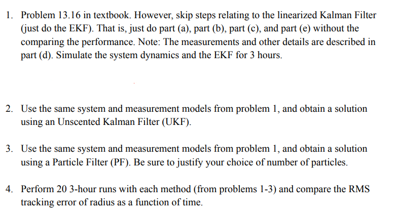
PLEASE SOLVE PART 3. You can use MATLAB or Python script

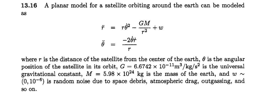
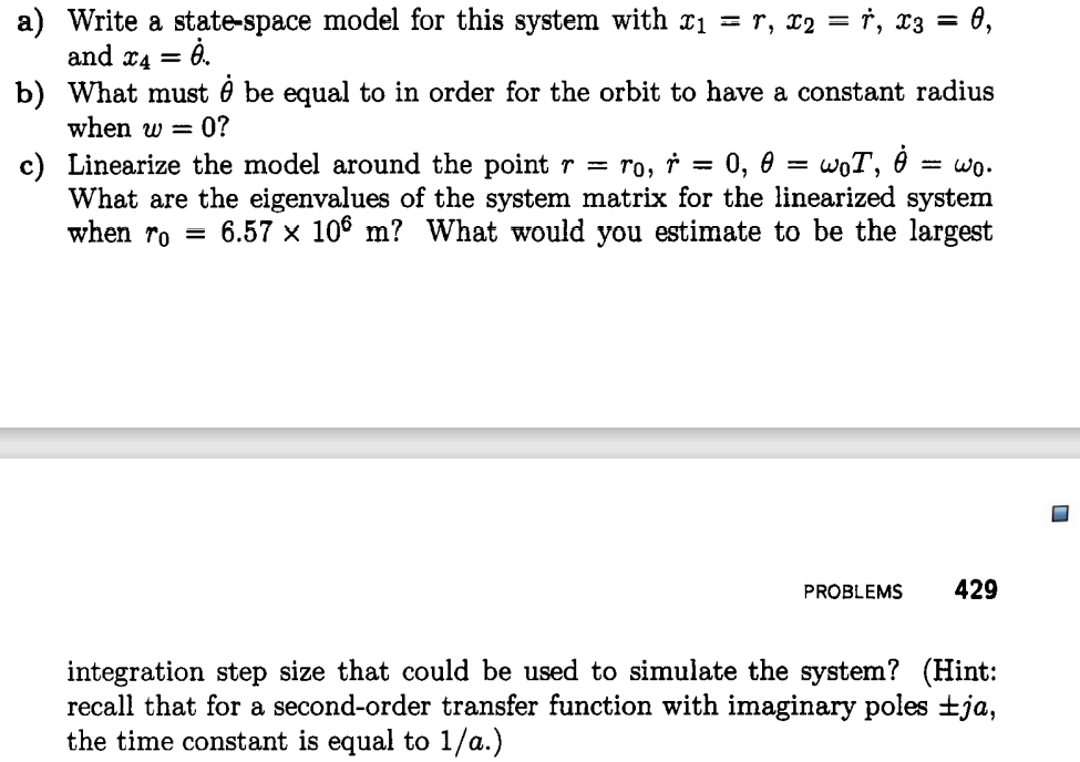
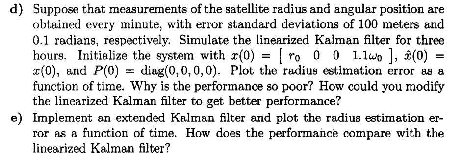
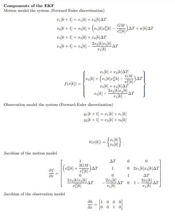
13.16 A planar model for a satellite orbiting around the earth can be modeled as r=r2r2GM+w=r2r where r is the distance of the satellite from the center of the earth, is the angular position of the satellite in its orbit, G=6.67421011m3/kg/s2 is the universal gravitational constant, M=5.981024kg is the mass of the earth, and w (0,106) is random noise due to space debris, atmospheric drag, outgassing, and so on. a) Write a state-space model for this system with x1=r,x2=r,x3=, and x4=. b) What must be equal to in order for the orbit to have a constant radius when w=0 ? c) Linearize the model around the point r=r0,r=0,=0T,=0. What are the eigenvalues of the system matrix for the linearized system when r0=6.57106m ? What would you estimate to be the largest 429 integration step size that could be used to simulate the system? (Hint: recall that for a second-order transfer function with imaginary poles ja, the time constant is equal to 1/a.) d) Suppose that measurements of the satellite radius and angular position are obtained every minute, with error standard deviations of 100 meters and 0.1 radians, respectively. Simulate the linearized Kalman filter for three hours. Initialize the system with x(0)=[r0001.10],x^(0)= x(0), and P(0)=diag(0,0,0,0). Plot the radius estimation error as a function of time. Why is the performance so poor? How could you modify the linearized Kalman filter to get better performance? e) Implement an extended Kalman filter and plot the radius estimation error as a function of time. How does the performance compare with the linearized Kalman filter? Components of the EKF Motion model the system (Forward Euler discretization) x1[k+1]=x1[k]+x2[k]Tx2[k+1]=x2[k]+(x1[k]x42[k]x12[k]GM)T+w[k]Tx3[k+1]=x3[k]+x4[k]Tx4[k+1]=x4[k]x1[k]2x2[k]x4[k]Tf(x[k])=x1[k]+x2[k]Tx2[k]+(x1[k]x42[k]x12[k]GM)Tx3[k]+x4[k]Tx4[k]x1[k]2x2[k]x4[k]T Observation model the system (Forward Euler discretization) y1[k+1]=x1[k]+vr[k]y2[k+1]=x3[k]+v[k] h(x[k])={x1[k]x3[k]} Jacobian of the motion model xf=1(x42[k]+x13[k]2GM)T0x12[k]2x2[k]x4[k]TT10x1[k]2x4[k]T001002x1[k]x4[k]TT1x1[k]2x2[k]T Jacobian of the observation model xh=[10000100] Problem 13.16 in textbook. However, skip steps relating to the linearized Kalman Filter (just do the EKF). That is, just do part (a), part (b), part (c), and part (e) without the comparing the performance. Note: The measurements and other details are described in part (d). Simulate the system dynamics and the EKF for 3 hours. 2. Use the same system and measurement models from problem 1, and obtain a solution using an Unscented Kalman Filter (UKF). Use the same system and measurement models from problem 1, and obtain a solution using a Particle Filter (PF). Be sure to justify your choice of number of particles. 4. Perform 20 3-hour runs with each method (from problems 1-3) and compare the RMS tracking error of radius as a function of time. 13.16 A planar model for a satellite orbiting around the earth can be modeled as r=r2r2GM+w=r2r where r is the distance of the satellite from the center of the earth, is the angular position of the satellite in its orbit, G=6.67421011m3/kg/s2 is the universal gravitational constant, M=5.981024kg is the mass of the earth, and w (0,106) is random noise due to space debris, atmospheric drag, outgassing, and so on. a) Write a state-space model for this system with x1=r,x2=r,x3=, and x4=. b) What must be equal to in order for the orbit to have a constant radius when w=0 ? c) Linearize the model around the point r=r0,r=0,=0T,=0. What are the eigenvalues of the system matrix for the linearized system when r0=6.57106m ? What would you estimate to be the largest 429 integration step size that could be used to simulate the system? (Hint: recall that for a second-order transfer function with imaginary poles ja, the time constant is equal to 1/a.) d) Suppose that measurements of the satellite radius and angular position are obtained every minute, with error standard deviations of 100 meters and 0.1 radians, respectively. Simulate the linearized Kalman filter for three hours. Initialize the system with x(0)=[r0001.10],x^(0)= x(0), and P(0)=diag(0,0,0,0). Plot the radius estimation error as a function of time. Why is the performance so poor? How could you modify the linearized Kalman filter to get better performance? e) Implement an extended Kalman filter and plot the radius estimation error as a function of time. How does the performance compare with the linearized Kalman filter? Components of the EKF Motion model the system (Forward Euler discretization) x1[k+1]=x1[k]+x2[k]Tx2[k+1]=x2[k]+(x1[k]x42[k]x12[k]GM)T+w[k]Tx3[k+1]=x3[k]+x4[k]Tx4[k+1]=x4[k]x1[k]2x2[k]x4[k]Tf(x[k])=x1[k]+x2[k]Tx2[k]+(x1[k]x42[k]x12[k]GM)Tx3[k]+x4[k]Tx4[k]x1[k]2x2[k]x4[k]T Observation model the system (Forward Euler discretization) y1[k+1]=x1[k]+vr[k]y2[k+1]=x3[k]+v[k] h(x[k])={x1[k]x3[k]} Jacobian of the motion model xf=1(x42[k]+x13[k]2GM)T0x12[k]2x2[k]x4[k]TT10x1[k]2x4[k]T001002x1[k]x4[k]TT1x1[k]2x2[k]T Jacobian of the observation model xh=[10000100] Problem 13.16 in textbook. However, skip steps relating to the linearized Kalman Filter (just do the EKF). That is, just do part (a), part (b), part (c), and part (e) without the comparing the performance. Note: The measurements and other details are described in part (d). Simulate the system dynamics and the EKF for 3 hours. 2. Use the same system and measurement models from problem 1, and obtain a solution using an Unscented Kalman Filter (UKF). Use the same system and measurement models from problem 1, and obtain a solution using a Particle Filter (PF). Be sure to justify your choice of number of particles. 4. Perform 20 3-hour runs with each method (from problems 1-3) and compare the RMS tracking error of radius as a function of time