Question

1 Approved Answer

Posted on Aug 01, 2024

////// Please Solve the questions using the outputs from stata given in the pictures ////// 1) in a panel data model with N=T=3, show and

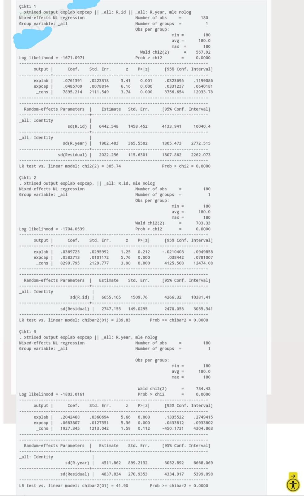
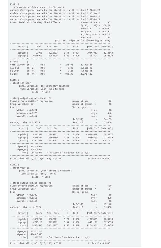
////// Please Solve the questions using the outputs from stata given in the pictures //////

1) in a panel data model with N=T=3, show and explain the operations you have made using a variance-covariance matrix, where you can create a simultaneous correlation between units, autocorrelation between first and second places, and heterogeneity in both units and in-unit.

2) the following production function of 9 companies is intended to be estimated using data from the period 2000-2017. Loutputit= Bo+B1 lexplapit+B2lexpcap+uit output: Logarithm of output quantity, lexplab: Logarithm of labor expenditures, and lexpcap: Logarithm of capital expenditures. Evaluate the following tests separately and together and decide on the appropriate model (test comments that do not write hypotheses will be invalid). Take a=0.05 for the tests.

image text in transcribed

180 kt 1 . xtmixed output explab expcap || _all: R.id || _all: R.year, mle nolog Mixed-effects ML regression Number of obs Group variable: _all Number of groups Obs per group: min = 1 180 avg = 180.0 max 180 Wald chi2(2) Prob > chi2 567.92 0.0000 Log likelihood -1671.0971 output Coef. Std. Err. Z P> 121 [95% Conf. Interval] .0761391 0223318 .0323695 . 1199086 explab exp | _cons 3.41 6.16 0.001 0.000 .0485709 .0078814 .0331237 .0640181 7895.214 2111.549 3.74 0.000 3756.654 12033.78 Random-effects parameters | Estimate Std. Err. [95% Conf. Interval] _all: Identity sd(R.id) 6442.548 1458.452 4133.941 10040.4 _all: Identity sd(R.year) | 1902.48 365.5502 1305.473 2772.515 sd (Residual) 2022.256 115.6301 1807.862 2262.073 LR test vs. linear model: chi2(2) = 305.74 Prob > chi2 = 0.0000 kt 2 xtmixed output explab expcap. ll _all: R.id, mle nolog Mixed-effects ML regression Number of obs Group variable: all Number of groups = Obs per group: min = 180 1 180 avg = 180.0 180 max = 703.33 Wald chi2(2) Prob > chi2 Log likelihood = -1704.0539 0.0000 output Coef. Std. Err. Z p>121 [95% Conf. Interval] .0369725 1.25 0.212 -.0210408 0949858 explab exp | cons .0295992 .0101172 .0582713 5.76 0.000 .038442 .0781007 8299.795 2129.777 3.90 0.000 4125.508 12474.08 Random-effects parameters Estimate Std. Err. [95% Conf. Interval] _all: Identity sd(R.id) 6655.105 1509.76 4266.32 10381.41 sd(Residual) 1 2747.155 149.0295 2470.055 3055.341 LR test vs. linear model: chibar2(01) = 239.83 Prob > chibar2 = 0.0000 kt 3 Xtmixed output explab expcap || _all: R.year, mle nolog Mixed-effects ML regression Number of obs Group variable: _all Number of groups 180 1 Obs per group: min = 180 avg = max = 180.0 180 784.43 Wald chi2(2) Prob > chi2 Log likelihood - -1803.0161 0.0000 output Coef. Std. Err. Z P> 121 (95% Conf. Interval] .0360694 5.66 0.000 . 1335522 explab expcap _cons . 2042468 .0683807 1927.345 .0127551 5.36 0.000 .0433812 .2749415 0933802 4304.863 1213.042 1.59 0.112 -450.1731 Random-effects parameters | Estimate Std. Err. [95% Conf. Interval) _all: Identity sd(R.year) 4511.862 899.2132 3052.892 6668.069 sd(Residual) 4837.834 270.9353 4334.917 5399.098 -> LR test vs. linear model: chibar2(01) = 41.90 Prob >= chibar2 = 0.0000 kti 4 twfe output explab expcap. Ids(id year) output: Convergence reached after iteration 1 with residual 3.2240e-20 explab: Convergence reached after iteration 1 with residual 3.2028e-20 expcap: Convergence reached after iteration 1 with residual 3.3204e-19 output: Convergence reached after iteration 1 with residual 1.3235e-21 Linear Model with Two-Way Fixed Effects Number of obs- 180 FC 30, 149) 209.24 Prob > 0.0000 R-squared = 0.9760 Adj R-squared - 0.9712 Root MSE 1864 (Std. Err. adjusted for clustering on none) output Coef. Std. Err. t Pit [95% Conf. Intervall .07963 .0226893 3.51 0.001 0347957 explab expcap . 1244643 .0636828 1 .0476919 .0080925 5.89 0.000 .031701 231.08 F-Test 1 Coefficients [ F2 All FES IF( 27 FE year F( 18, FE idi IF( 10, 8.05 149) 149) 149) 149) 2.157e-46 5.565e-18 1.553e-16 2.27e-129 9.21 945.30 kt 5 . xtset Id1 year panel variable: 1dl (strongly balanced) time variable: year. 1966 to 1963 delta: 1 unit - 180 10 Xtreg output explab expcap, fe Fixed-effects (within) regression Group variable: idi R-Sq: within = 0.8021 between = 0.9575 overall = 0.7341 = Number of obs Number of groups Obs per group min 18 avg 18.0 max - 18 340.55 F(2,168) Prob > F corru, Xb) = 0.5515 0.0000 output Coef. Std. Err. t Pit [95% Conf. Intervall explab .0342359 .0299312 1.14 0.254 -.0248539 .0933257 exp 1 .0586302 .0102289 5.73 0.000 .0384365 .0788239 _cons 8356.807 329.4041 25.37 0.000 7706.502 9007. 112 - sigma_u! 7083.4989 sigma_e) 2763.0524 rho 86793974 (fraction of variance due to 1) F test that all u_1=0: F(9, 168) = 78.46 9, ) Prob > F = 0.0000 akt 6 xtset year idi panel variable: year (strongly balanced) time variable: id, 1 to 10 delta: 1 unit 180 18 xtreg output explab expcap, fe Fixed-effects (within) regression Group variable: year R-59: within = 0.8302 between = 0.8266 overall - 0.7442 Number of obs Number of groups - Obs per group: min 10 10.0 avg - max 2 10 391.26 corr(u 1, Xb) F(2,160) Prob > -0.6125 0.0000 output Coef. Std. Err. t pit [95% Conf. Interval) --------------- 2088264 .0362021 5.77 0.000 . 1373309 explab expcap _cons 1 .0725118 .0128582 .0471181 5.64 0.000 2.35 0.020 2803218 .0979055 2588.78 1405.536 599.1407 222.2924 sigma_u 5237.2215 sigma_e | 4849.5906 rho .5383728 (fraction of variance due to ui) F test that all u_1=0: F(17, 160) = 7.28 Prob > F = 0.0000 180 kt 1 . xtmixed output explab expcap || _all: R.id || _all: R.year, mle nolog Mixed-effects ML regression Number of obs Group variable: _all Number of groups Obs per group: min = 1 180 avg = 180.0 max 180 Wald chi2(2) Prob > chi2 567.92 0.0000 Log likelihood -1671.0971 output Coef. Std. Err. Z P> 121 [95% Conf. Interval] .0761391 0223318 .0323695 . 1199086 explab exp | _cons 3.41 6.16 0.001 0.000 .0485709 .0078814 .0331237 .0640181 7895.214 2111.549 3.74 0.000 3756.654 12033.78 Random-effects parameters | Estimate Std. Err. [95% Conf. Interval] _all: Identity sd(R.id) 6442.548 1458.452 4133.941 10040.4 _all: Identity sd(R.year) | 1902.48 365.5502 1305.473 2772.515 sd (Residual) 2022.256 115.6301 1807.862 2262.073 LR test vs. linear model: chi2(2) = 305.74 Prob > chi2 = 0.0000 kt 2 xtmixed output explab expcap. ll _all: R.id, mle nolog Mixed-effects ML regression Number of obs Group variable: all Number of groups = Obs per group: min = 180 1 180 avg = 180.0 180 max = 703.33 Wald chi2(2) Prob > chi2 Log likelihood = -1704.0539 0.0000 output Coef. Std. Err. Z p>121 [95% Conf. Interval] .0369725 1.25 0.212 -.0210408 0949858 explab exp | cons .0295992 .0101172 .0582713 5.76 0.000 .038442 .0781007 8299.795 2129.777 3.90 0.000 4125.508 12474.08 Random-effects parameters Estimate Std. Err. [95% Conf. Interval] _all: Identity sd(R.id) 6655.105 1509.76 4266.32 10381.41 sd(Residual) 1 2747.155 149.0295 2470.055 3055.341 LR test vs. linear model: chibar2(01) = 239.83 Prob > chibar2 = 0.0000 kt 3 Xtmixed output explab expcap || _all: R.year, mle nolog Mixed-effects ML regression Number of obs Group variable: _all Number of groups 180 1 Obs per group: min = 180 avg = max = 180.0 180 784.43 Wald chi2(2) Prob > chi2 Log likelihood - -1803.0161 0.0000 output Coef. Std. Err. Z P> 121 (95% Conf. Interval] .0360694 5.66 0.000 . 1335522 explab expcap _cons . 2042468 .0683807 1927.345 .0127551 5.36 0.000 .0433812 .2749415 0933802 4304.863 1213.042 1.59 0.112 -450.1731 Random-effects parameters | Estimate Std. Err. [95% Conf. Interval) _all: Identity sd(R.year) 4511.862 899.2132 3052.892 6668.069 sd(Residual) 4837.834 270.9353 4334.917 5399.098 -> LR test vs. linear model: chibar2(01) = 41.90 Prob >= chibar2 = 0.0000 kti 4 twfe output explab expcap. Ids(id year) output: Convergence reached after iteration 1 with residual 3.2240e-20 explab: Convergence reached after iteration 1 with residual 3.2028e-20 expcap: Convergence reached after iteration 1 with residual 3.3204e-19 output: Convergence reached after iteration 1 with residual 1.3235e-21 Linear Model with Two-Way Fixed Effects Number of obs- 180 FC 30, 149) 209.24 Prob > 0.0000 R-squared = 0.9760 Adj R-squared - 0.9712 Root MSE 1864 (Std. Err. adjusted for clustering on none) output Coef. Std. Err. t Pit [95% Conf. Intervall .07963 .0226893 3.51 0.001 0347957 explab expcap . 1244643 .0636828 1 .0476919 .0080925 5.89 0.000 .031701 231.08 F-Test 1 Coefficients [ F2 All FES IF( 27 FE year F( 18, FE idi IF( 10, 8.05 149) 149) 149) 149) 2.157e-46 5.565e-18 1.553e-16 2.27e-129 9.21 945.30 kt 5 . xtset Id1 year panel variable: 1dl (strongly balanced) time variable: year. 1966 to 1963 delta: 1 unit - 180 10 Xtreg output explab expcap, fe Fixed-effects (within) regression Group variable: idi R-Sq: within = 0.8021 between = 0.9575 overall = 0.7341 = Number of obs Number of groups Obs per group min 18 avg 18.0 max - 18 340.55 F(2,168) Prob > F corru, Xb) = 0.5515 0.0000 output Coef. Std. Err. t Pit [95% Conf. Intervall explab .0342359 .0299312 1.14 0.254 -.0248539 .0933257 exp 1 .0586302 .0102289 5.73 0.000 .0384365 .0788239 _cons 8356.807 329.4041 25.37 0.000 7706.502 9007. 112 - sigma_u! 7083.4989 sigma_e) 2763.0524 rho 86793974 (fraction of variance due to 1) F test that all u_1=0: F(9, 168) = 78.46 9, ) Prob > F = 0.0000 akt 6 xtset year idi panel variable: year (strongly balanced) time variable: id, 1 to 10 delta: 1 unit 180 18 xtreg output explab expcap, fe Fixed-effects (within) regression Group variable: year R-59: within = 0.8302 between = 0.8266 overall - 0.7442 Number of obs Number of groups - Obs per group: min 10 10.0 avg - max 2 10 391.26 corr(u 1, Xb) F(2,160) Prob > -0.6125 0.0000 output Coef. Std. Err. t pit [95% Conf. Interval) --------------- 2088264 .0362021 5.77 0.000 . 1373309 explab expcap _cons 1 .0725118 .0128582 .0471181 5.64 0.000 2.35 0.020 2803218 .0979055 2588.78 1405.536 599.1407 222.2924 sigma_u 5237.2215 sigma_e | 4849.5906 rho .5383728 (fraction of variance due to ui) F test that all u_1=0: F(17, 160) = 7.28 Prob > F = 0.0000