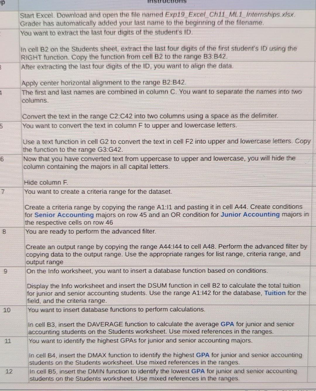
please solve this is excel

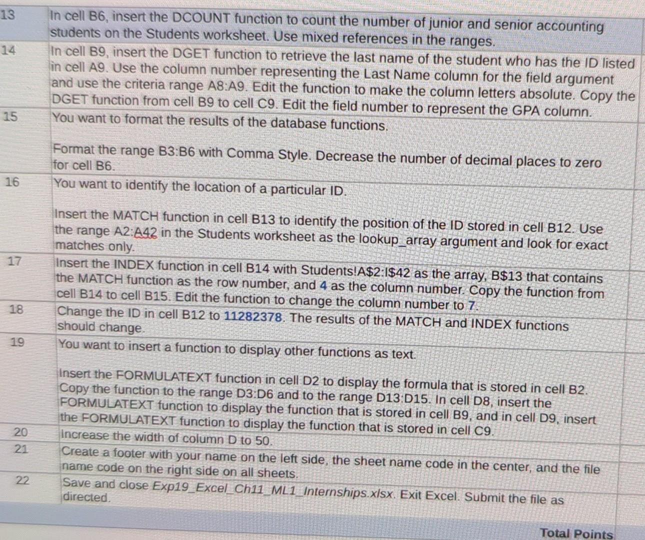
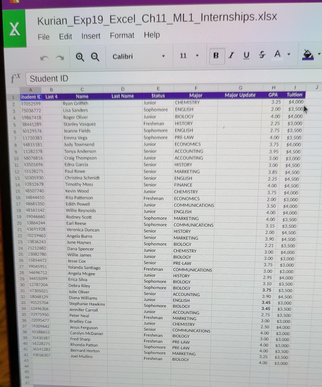
ep Start Excel. Download and open the file named Exp19_Excel_Ch11_ML1_Internships xlsx Grader has automatically added your last name to the beginning of the filename. You want to extract the last four digits of the student's ID. In cell B2 on the Students sheet, extract the last four digits of the first student's ID using the RIGHT function. Copy the function from cell B2 to the range B3.842. After extracting the last four digits of the ID, you want to align the data. 3 4 Apply center horizontal alignment to the range B2:B42. The first and last names are combined in column C. You want to separate the names into two columns Convert the text in the range C2:C42 into two columns using a space as the delimiter You want to convert the text in column F to upper and lowercase letters. 5 Use a text function in cell G2 to convert the text in cell F2 into upper and lowercase letters. Copy the function to the range G3:G42. Now that you have converted text from uppercase to upper and lowercase, you will hide the column containing the majors in all capital letters. 6 7 Hide column F. You want to create a criteria range for the dataset. Create a criteria range by copying the range A1:11 and pasting it in cell A44. Create conditions for Senior Accounting majors on row 45 and an OR condition for Junior Accounting majors in the respective cells on row 46 You are ready to perform the advanced filter. 8. Create an output range by copying the range A44:144 to cell A48. Perform the advanced filter by copying data to the output range. Use the appropriate ranges for list range, criteria range, and output range On the Info worksheet, you want to insert a database function based on conditions. 9 Display the Info worksheet and insert the DSUM function in cell B2 to calculate the total tuition for junior and senior accounting students. Use the range A1:142 for the database, Tuition for the field, and the criteria range. You want to insert database functions to perform calculations. 10 In cell B3, insert the DAVERAGE function to calculate the average GPA for junior and senior accounting students on the Students worksheet. Use mixed references in the ranges. You want to identify the highest GPAs for junior and senior accounting majors. 11 In cell B4, insert the DMAX function to identify the highest GPA for junior and senior accounting students on the Students worksheet. Use mixed references in the ranges. In cell B5, insert the DMIN function to identify the lowest GPA for junior and senior accounting students on the Students worksheet. Use mixed references in the ranges. 12 13 14 In cell B6, insert the DCOUNT function to count the number of junior and senior accounting students on the Students worksheet. Use mixed references in the ranges. In cell B9, insert the DGET function to retrieve the last name of the student who has the ID listed in cell A9. Use the column number representing the Last Name column for the field argument and use the criteria range A8:A9. Edit the function to make the column letters absolute. Copy the DGET function from cell B9 to cell C9. Edit the field number to represent the GPA column. You want to format the results of the database functions. 15 Format the range B3:B6 with Comma Style. Decrease the number of decimal places to zero for cell B6. You want to identify the location of a particular ID. 16 17 Insert the MATCH function in cell B13 to identify the position of the ID stored in cell B12. Use the range A2:A42 in the Students worksheet as the lookup_array argument and look for exact matches only Insert the INDEX function in cell B14 with Students!A$2:1$42 as the array, B$13 that contains the MATCH function as the row number, and 4 as the column number. Copy the function from cell B14 to cell B15. Edit the function to change the column number to 7. Change the ID in cell B12 to 11282378. The results of the MATCH and INDEX functions should change You want to insert a function to display other functions as text. 18 19 20 Insert the FORMULATEXT function in cell D2 to display the formula that is stored in cell B2. Copy the function to the range D3 D6 and to the range D13:015. In cell D8, insert the FORMULATEXT function to display the function that is stored in cell B9, and in cell D9, insert the FORMULATEXT function to display the function that is stored in cell C9. increase the width of column D to 50. Create a footer with your name on the left side, the sheet name code in the center, and the file name code on the right side on all sheets. Save and close Exp19 Excel_Ch11_ML1_Internships.xlsx. Exit Excel. Submit the file as directed 21 22 Total Points X Kurian_Exp19_ExcelCh11_ML1_Internships.xlsx Edit Insert Format Help File @ @ Calibri 11 BI U A. fx Student ID J D Last Name A B 1 Student IC Last 4 2 97052599 3 75036772 4 59867418 5 38441289 6 50129576 7 11720383 8 44815181 9 11282378 10 56076816 11 43501696 12 55128275 13 50305930 14 92812678 15 48507740 16 34844410 17 48681350 18 48161142 19 39046660 20 33864244 21 43691928 22 70219463 23 53836243 24 21212682 25 23082780 26 55854472 27 99045951 28 54696712 29 34455099 30 12787204 31 47305021 32 18068129 33 90525704 34 52496306 35 92975950 36 22095477 37 59309642 50188653 35430187 40 56228275 36141283 42 93036307 43 Name Ryan Griffith Lisa Sanders Roger Oliver Stanley Vasquez Jeanne Fields Emma Vega Judy Townsend Tonya Anderson Craig Thompson Edna Garcia Paul Rowe Christina Schmidt Timothy Moss Kevin Wood Rita Patterson Edith Powell Willie Reynolds Rodney Scott Earl Reese Veronica Duncan Angela Burns June Haynes Dana Spencer Willie James Jesse Cox Yolanda Santiago Angela Mcgee Erica Silva Debra Riley Julie Oliver Diana Williams Stephanie Hawkins Jennifer Carroll Peter Neal Bradley Cox Jesus Ferguson Carolyn McDaniel Fred Sharp Rhonda Patton Bernard Horton Joel Mullins E Status Major Junior CHEMISTRY Sophomore ENGLISH Junior BIOLOGY Freshman HISTORY Sophomore ENGLISH Sophomore PRE-LAW Junior ECONOMICS Senior ACCOUNTING Junior ACCOUNTING Senior HISTORY Senior MARKETING Senior ENGLISH Senior FINANCE Junior CHEMISTRY Freshman ECONOMICS Junior COMMUNICATIONS Junior ENGLISH Sophomore MARKETING Sophomore COMMUNICATIONS Senior HISTORY Senior MARKETING Sophomore BIOLOGY Junior CHEMISTRY Junior BIOLOGY Senior PRE-LAW Freshman COMMUNICATIONS Junior HISTORY Sophomore BIOLOGY Sophomore BIOLOGY Senior ACCOUNTING Junior ENGLISH Sophomore BIOLOGY Junior ACCOUNTING Freshman MARKETING Junior CHEMISTRY Senior COMMUNICATIONS Freshman BIOLOGY Freshman PRE-LAW Sophomore PRE-LAW Sophomore MARKETING Freshman BIOLOGY G H Major Update GPA Tuition 3.25 $4,000 2.00 $3,500 4.00 $4,000 2.25 $3,000 2.75 $3,500 4.00 $3,500 3.75 $4,000 3.95 $4,500 3.00 $3,000 3.00 $4,500 3.85 $4,500 2.25 $4.500 4.00 $4,500 3.75 $4,000 2.00 $3,000 3.50 $4,000 4.00 $4,000 4.00 $3,500 3.15 $3,500 2.00 $4,500 3.90 $4,500 2.21 $3,500 3.00 $4,000 3.00 $3,000 $3,000 3.00 $3,000 2.95 $4,000 3.10 $3,500 3.75 $3,500 3.90 $4,500 3.45 $3,000 3.45 $3,500 $3,500 3.00 $3.000 2.50 $4,000 4.00 $3,000 3.00 $3,000 4.00 $3,000 4.00 $3,500 3.25 $3,500 4.00 $3,000 3.75 2.75 44 45 46 49