Please solve this question in Matlab. Thanks!

And the natspline.m code is:

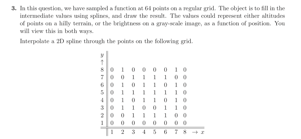
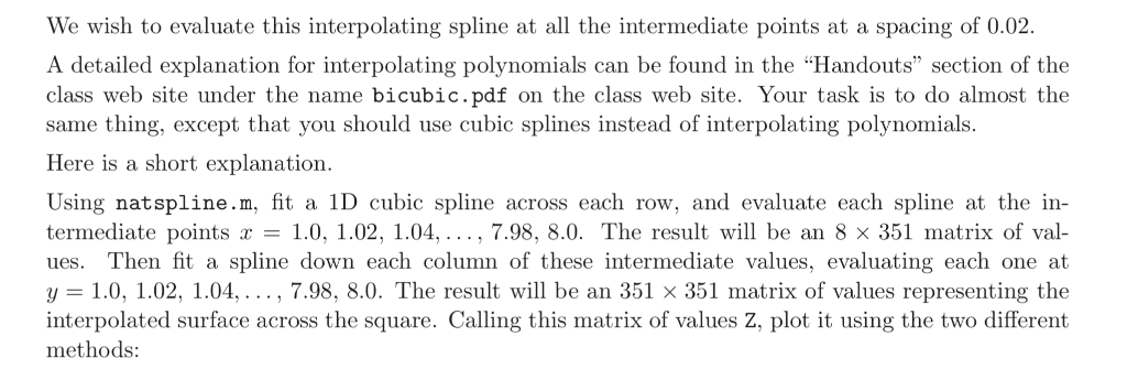
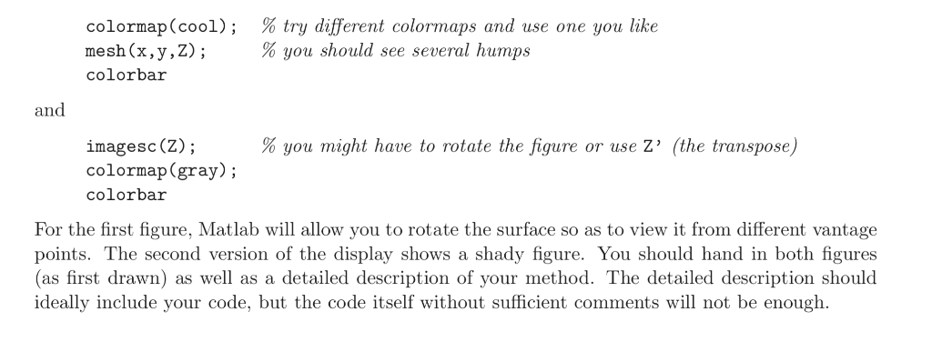
function pp = natspline(x,y,conds) %CSAPE Cubic spline interpolation with various end conditions. % Default changed to be the 'natural' cubic spline (2nd deriv's == 0 at ends) % % PP = CSAPE(X,Y) returns the cubic spline interpolant (in ppform) to the % given data (X,Y) using Lagrange end conditions (the default in table below). % The interpolant matches, at the data site X(j), the given data value % Y(:,j), j=1:length(X). The data values may be scalars, vectors. % % PP = CSAPE(X,Y,CONDS) uses the end conditions specified by CONDS, with % corresponding end condition values endcondvals . % If there are two more data values than data sites, then the first (last) % data value is taken as the value for the left (right) end condition, i.e., % endcondvals = Y(:,[1 end]). % Otherwise, default values are used. % % CONDS may be a *string* whose first character matches one of the % following: 'complete' or 'clamped', 'periodic', % 'second', 'variational', with the following meanings: % % 'complete' : match endslopes to the slope of the cubic that % matches the first four data at the respective end. % 'not-a-knot' : no longer supported by this function. % 'periodic' : match first and second derivatives at first data % point with those at last data point % (ignoring given end condition values if any) % 'second' : match end second derivatives (as given, % with default [0 0], i.e., as in variational) % 'variational' : set end second derivatives equal to zero % (ignoring given end condition values if any) % The *default* : natural cubic spline (like 'second' w/ zero end conditions) % % By giving CONDS as a 1-by-2 matrix instead, it is possible to % specify *different* conditions at the two endpoints, namely % CONDS(i) with value endcondvals(:,i), with i=1 (i=2) referring to the % left (right) endpoint. % % CONDS(i)=j means that the j-th derivative is being specified to % be endcondvals(:,i) , j=1,2. CONDS(1)=0=CONDS(2) means periodic end % conditions. % % If CONDS(i) is not specified or is different from 0, 1 or 2, then % the default value for CONDS(i) is 1 and the default value of % endcondvals(:,i) is taken. If no end condition values are specified, % then the default value for endcondvals(:,i) is taken to be % % deriv. of cubic interpolant to nearest four points, if CONDS(i)=1; % 0 if CONDS(i)=2. % % For example, % % x = linspace(0,2*pi,9); %% sample every 45 degrees. % pp = natspline( x, [1 sin(x) 0], [1 2] ); % xx=linspace(0,2*pi,50); %% many samples for drawing curve. % plot(xx,ppval(pp,xx)); % % gives a good approximation to the sine function on the interval [0 .. 2*pi] % (matching its slope 1 at the left endpoint, x(1) = 0, and its second % derivative 0 at the right endpoint, x(9) = 2*pi, in addition to its value % at every x(i), i=1:9). % % The following plots a circle: % % x = [0:.1:4]; pp=natspline( [0:4], [1 0 -1 0 1;0 1 0 -1 0], 'periodic'); % y = ppval(pp,x); plot(y(1,:),y(2,:)); axis equal; % % Copyright 1987-2003 C. de Boor and The MathWorks, Inc. % $Revision: 1.23 $ editted for use in UofM class % Generate the cubic spline interpolant in ppform. if nargin2, ddf=(divdif(2,:)-divdif(1,:))/(xi(3)-xi(1)); b(1,:) = b(1,:)-ddf*dx(1); end if n>3, ddf2=(divdif(3,:)-divdif(2,:))/(xi(4)-xi(2)); b(1,:)=b(1,:)+(ddf2-ddf)*(dx(1)*(xi(3)-xi(1)))/(xi(4)-xi(1)); end end end if ~any(conds) c(n,1:2)=dx(n-1)*[2 1]; c(n,n-1:n)= c(n,n-1:n)+dx(1)*[1 2]; b(n,:) = 3*(dx(n-1)*divdif(1,:) + dx(1)*divdif(n-1,:)); elseif conds(2)==2 c(n,n-1:n)=[1 2]; b(n,:)=3*divdif(n-1,:)+(dx(n-1)/2)*valconds(:,2).'; else c(n,n-1:n) = [0 1]; b(n,:) = valconds(:,2).'; if ((valsnotgiven)||(conds(2)~=1)) % if endslope was not supplied, % get it by local interpolation b(n,:)=divdif(n-1,:); if n>2, ddf=(divdif(n-1,:)-divdif(n-2,:))/(xi(n)-xi(n-2)); b(n,:) = b(n,:)+ddf*dx(n-1); end if n>3, ddf2=(divdif(n-2,:)-divdif(n-3,:))/(xi(n-1)-xi(n-3)); b(n,:)=b(n,:)+(ddf-ddf2)*(dx(n-1)*(xi(n)-xi(n-2)))/(xi(n)-xi(n-3)); end end end % solve for the slopes .. (protect current spparms setting) mmdflag = spparms('autommd'); spparms('autommd',0); % suppress pivoting s=c\b; spparms('autommd',mmdflag); % .. and convert to ppform c4 = (s(1:n-1,:)+s(2:n,:)-2*divdif(1:n-1,:))./dx(:,dd); c3 = (divdif(1:n-1,:)-s(1:n-1,:))./dx(:,dd) - c4; pp = mkpp(xi.', ... reshape([(c4./dx(:,dd)).' c3.' s(1:n-1,:).' yi(1:n-1,:).'],(n-1)*yd,4),yd); if length(sizeval)>1, pp = fnchg(pp,'dz',sizeval); end if ~isfield(pp,'coefs');pp.coefs=pp.P;end;

3. In this question, we have sampled a function at 64 points on a regular grid. The object is to fill in the intermediate values using splines, and draw the result. The values could represent either altitudes of points on a hilly terrain, or the brightness on a gray-scale image, as a function of position. You will view this in both ways. Interpolate a 2D spline through the points on the following grid. 60 1 0 1 0 10 345678X We wish to evaluate this interpolating spline at all the intermediate points at a spacing of 0.02 A detailed explanation for interpolating polynomials can be found in the "Handouts" section of the class web site under the name bicubic.pdf on the class web site. Your task is to do almost the same thing, except that you should use cubic splines instead of interpolating polynomials. Here is a short explanation. Using natspline.m, fit a 1D cubic spline across each row, and evaluate each spline at the in termediate points x-1.0, 1.02, 1.04, , 7.98, 8.0. The result will be an 8 351 matrix of val- ues. Then fit a spline down each column of these intermediate values, evaluating each one at y 1.0, 1.02, 1.04,.., 7.98, 8.0. The result will be an 351 x 351 matrix of values representing the interpolated surface across the square. Calling this matrix of values Z, plot it using the two different methods: colormap (cool) mesh(x,y,2); colorbar % try different colormaps and use one you like % you should see several humps ; and % you might have to rotate the figure or use Z' (the transpose) imagesc(Z); colormap (gray); colorbar For the first figure, Matlab will allow you to rotate the surface so as to view it from different vantage points. The second version of the display shows a shady figure. You should hand in both figures (as first drawn) as well as a detailed description of your method. The detailed description shoulod ideally include your code, but the code itself without sufficient comments will not be enough 3. In this question, we have sampled a function at 64 points on a regular grid. The object is to fill in the intermediate values using splines, and draw the result. The values could represent either altitudes of points on a hilly terrain, or the brightness on a gray-scale image, as a function of position. You will view this in both ways. Interpolate a 2D spline through the points on the following grid. 60 1 0 1 0 10 345678X We wish to evaluate this interpolating spline at all the intermediate points at a spacing of 0.02 A detailed explanation for interpolating polynomials can be found in the "Handouts" section of the class web site under the name bicubic.pdf on the class web site. Your task is to do almost the same thing, except that you should use cubic splines instead of interpolating polynomials. Here is a short explanation. Using natspline.m, fit a 1D cubic spline across each row, and evaluate each spline at the in termediate points x-1.0, 1.02, 1.04, , 7.98, 8.0. The result will be an 8 351 matrix of val- ues. Then fit a spline down each column of these intermediate values, evaluating each one at y 1.0, 1.02, 1.04,.., 7.98, 8.0. The result will be an 351 x 351 matrix of values representing the interpolated surface across the square. Calling this matrix of values Z, plot it using the two different methods: colormap (cool) mesh(x,y,2); colorbar % try different colormaps and use one you like % you should see several humps ; and % you might have to rotate the figure or use Z' (the transpose) imagesc(Z); colormap (gray); colorbar For the first figure, Matlab will allow you to rotate the surface so as to view it from different vantage points. The second version of the display shows a shady figure. You should hand in both figures (as first drawn) as well as a detailed description of your method. The detailed description shoulod ideally include your code, but the code itself without sufficient comments will not be enough