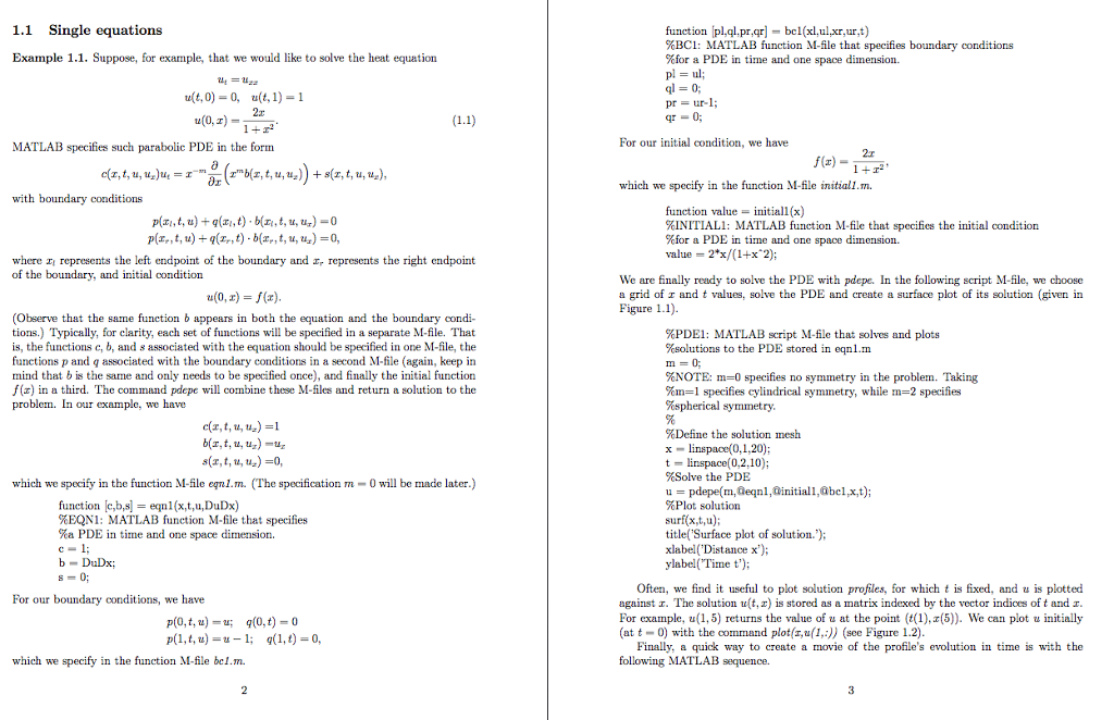
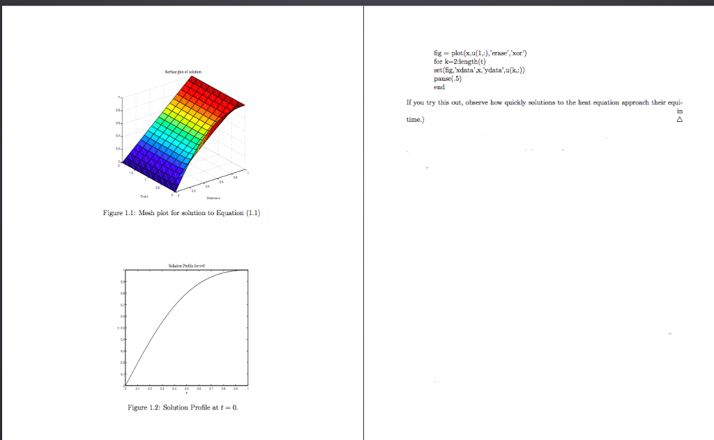
Please try to re-write the matlab codes in clear and nice way because I could not get the last two figures by using the written codes. I want the codes that give me the last two figures:

1.1 Single equations function [pl,ql.pr qr] bel(xl,ul.xr,ur,t) %BC1: MATLAB function M-file that specifies boundary conditions %for a PDE in time and one space dimension. Example 1.1. Suppose, for example, that e wuld like to solve the heat equation l-0; pr = ur-l; 2r: u(0,) MATLAB specifies such parabolic PDE in the form For o tial condition, we have ,t,u, )utu,)+(r,t,u,u.) which we specify in the function Mfile initiall.m. with boundary conditions Pi,t,)g(x,t) bt u u-0 Plz, , t, tl)-q(z,, t) . b(z, , t, u, u.) = 0, function value initiall(x) %INITIAL 1: MATLAB function M-file that specifies the initial condition %for a PDE in time and one space dimension. value 2*x/(1+x 2) where x of the boundarv, and initial condition represents the left endpoint of the boundary and represents the right endpoint We are finally ready to solve the PDE with pdepe. In the following script M-file, we choose a grid of r and t values, solve the PDE and create a surface plot of its solution (given in Figure 1.1). u(0, ( (Observe that the same function b appears in both the equation and the boundary condi- tions.) Typically, for clarity, each set offunctions will be specified in a separate M-file. That is, the functions c, b, and s associated with the equation should be specified in one M-file, the functions p and q associated with the boundary conditions in a second M-file (again, keep in mind that b is the same and only needs to be specified once), and finally the initial function f(z) in a third. The command pdepe will combine these M-files and return a solution to the %PDE1: MATLAB script M-file that solves and plots %solutions to the PDE stored in eqn1.m %NOTE: m-0 specifies no symmetry in the problem. Taking %m-1 specifies cylindrical symmetry, while m 2 specifies %spherical symmetry problem. In our example, we have c(r, t, u, uz)-1 %Define the solution mesh x-linspace(0,1,20; t- linspace (0,2,10); %Solve the PDE u- pdepe(m, eqn1,0initial,abel,x,t); %Plot solution surfx,t,u); titlelSurface plot of solution.'); xlabel('Distance x); ylabel(Time t'; s(r, t, u,u)0, which we spocify in the function M-file eqml.m. The specification 0 will be made later.) function c,b,selx,t,u,DuDx) %EQNI: MATLAB function M-file that specifies %a PDE in time and one space dimension. b DuD; Often, we find it useful to plot solution profiles, for which t is fixed, and u is plotted against r. The solution u(t, z) is stored as a matrix indexed by the vector indices of t and r. For example, u(1,5) returns the value of at the point (t(1),x(5)). We can plot nitially (at t-0) with the command plotfr,u(1,:)) (see Figure 1.2) For our boundary conditions, we have p(0,t,u)=u; q(0,t) = 0 Finally, a quick way to create a movie of the profile's evolution in time is with the following MATLAB sequence. which we specify in the function M-file bel.m fig-plotxu(1,),erase','xor) for k-2 length(t) set (fig,'xdata''ydata",u(k)) pause(-5) end If you try this out, observe how quickly solutions to the heat equation approach theirequi in time.) Figure 1.1: Mesh plot for solution to Equation1.1) Figure 12: Solution Profile at t-0