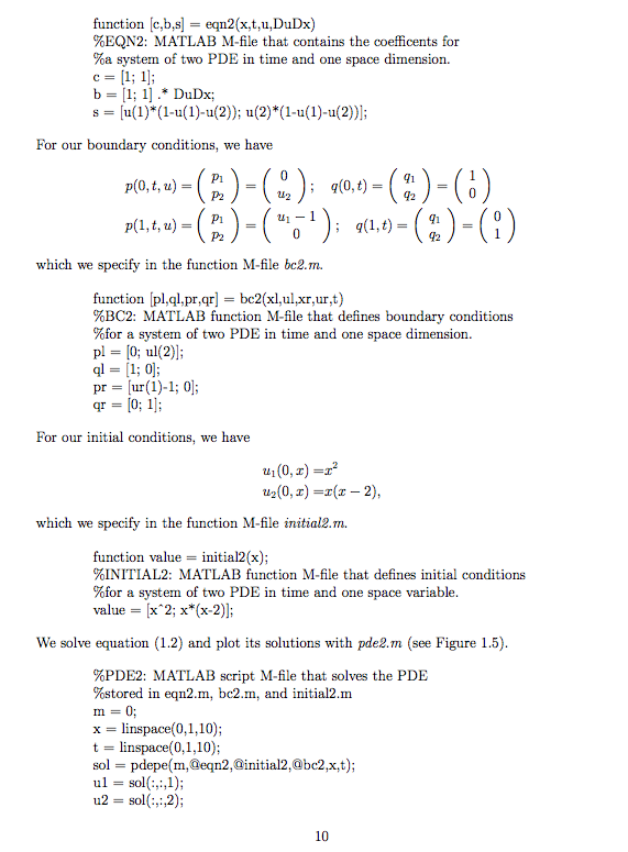
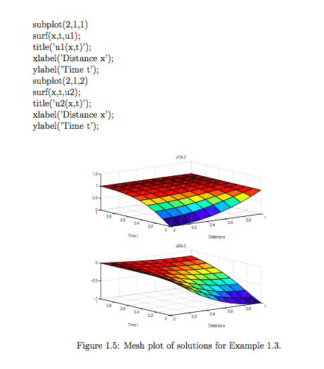
Please try to re-write the matlab codes in clear and nice way because I could not get the last two figures by using the written codes. I want the codes that give me the last two figures:

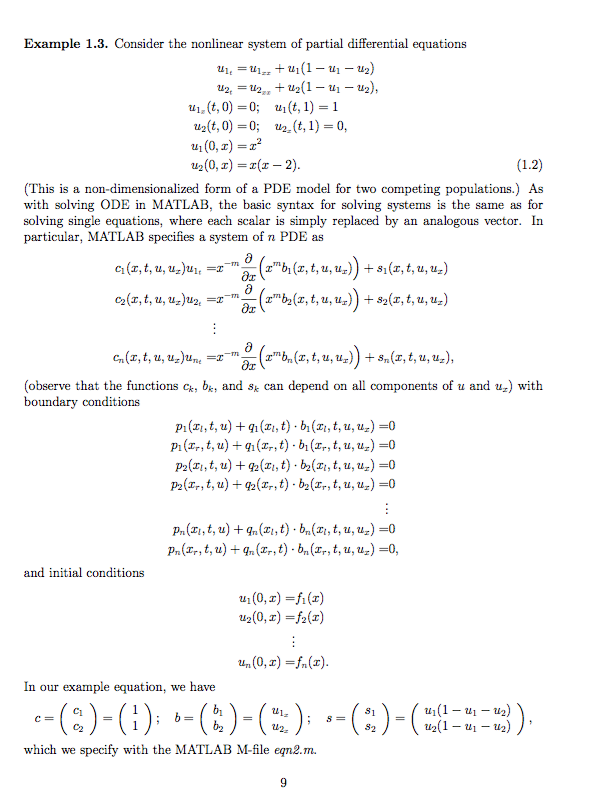
Example 1.3. Consider the nonlinear system of partial differential equations u2(0,)(x -2). (This is a non-di with solving ODE in MATLAB, the basic syntax for solving systems is the same as for solving single equations, where each scalar is simply replaced by an analogous vector. In particular, MATLAB specifies a system of n PDE as form of a PDE model for two competing populations.) As ,t, u, u,st,,) (observe that the functions ck, bk, and sk can depend on all components of u and u) with boundary conditions pi(i,t,u +gi(zi,t) b(,t, u, ur)0 Pi(x, t, u)+g(,t) btu, u)-0 p2(r, t, u+(r,t) b2(xr, t,u, ur)0 Pn(z,, t, u) + gn(z,, t) . bn (zr, t, u, uz) =0, and initial conditions ui (0,z) =A(z) m(0,z) = (z) In our example equation, we have u(1-u2) 21-u-2) which we specify with the MATLAB M-file eqn2.m. function [c,b,s-eqn2(x,t,u,DuDx) %EQN2 : MATLAB M-file that contains the coefficents for %a system of two PDE in time and one space dimension. For our boundary conditions, we have p(0,t,u)=( P1 p(l, t, u) P which we specify in the function M-file bc2.m. function [pl,ql.pr,qr]bc2(xl,ul.xr,ur,t) %BC2: MATLAB function M-file that defines boundary conditions %for a system of two PDE in time and one space dimension. pl- [0; ul(2); pr = [ur( 1)-1; For our initial conditions, we have u2(0, x -2), which we specify in the function M-file initial2.m. function value initial2(x); %INITIAL2: MATLAB function M-file that defines initial conditions %for a system of two PDE in time and one space variable value x 2; x*(x-2)]; We solve equation (1.2) and plot its solutions with pde2.m (see Figure 1.5) %PDE2: MATLAB script M-file that solves the PDE %stored in eqn2.m, be2m, and initia!2.m m-0; x linspace(0,1,10); t inspace(0,1,10); sol-pdepe(m, @eqn2,@initial2,@bc2,x,t); ul - sol(:,:,1); u2 = sol(:,:,2); 10 subplot(2,1,1) surf(x,t,ul) title('ul(x,t)"); xlabel(Distance x'); ylabel(Time t); subplot(2,1,2) surf(x,t,u2) title('u2(x,t)"); xlabel(Distance x'); ylabel(Time t); 05 0.5 02 0.5 02 Figure 1.5: Mesh plot of solutions for Example 1.3