please use excel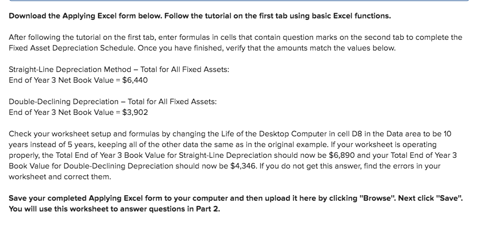

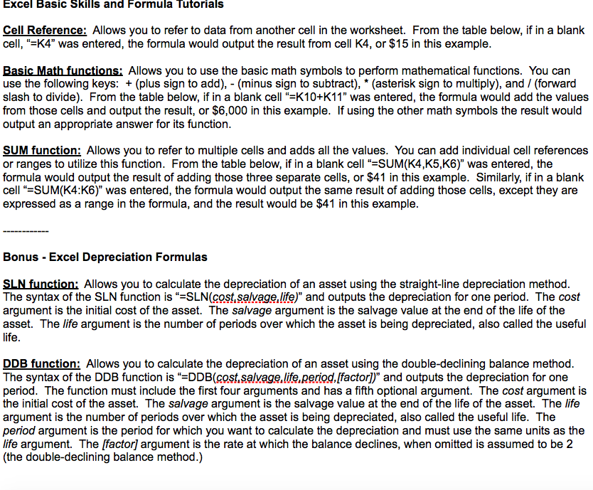
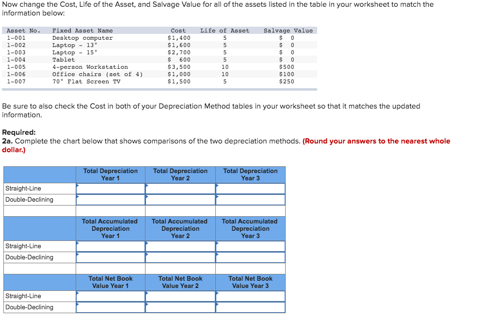
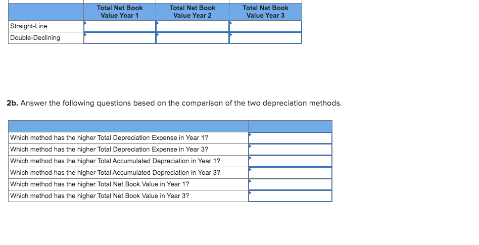
Download the Applying Excel form below. Follow the tutorial on the first tab using basic Excel functions. After following the tutorial on the first tab, enter formulas in cells that contain question marks on the second tab to complete the Fixed Asset Depreciation Schedule. Once you have finished, verify that the amounts match the values below. Straight-Line Depreciation Method - Total for All Fixed Assets: End of Year 3 Net Book Value = $6,440 Double-Declining Depreciation - Total for All Fixed Assets: End of Year 3 Net Book Value = $3,902 Check your worksheet setup and formulas by changing the Life of the Desktop Computer in cell D8 in the Data area to be 10 years instead of 5 years, keeping all of the other data the same as in the original example. If your worksheet is operating properly, the Total End of Year 3 Book Value for Straight-Line Depreciation should now be $6,890 and your Total End of Year 3 Book Value for Double-Declining Depreciation should now be $4,346. If you do not get this answer, find the errors in your worksheet and correct them. Save your completed Applying Excel form to your computer and then upload it here by clicking "Browse". Next click "Save". You will use this worksheet to answer questions in Part 2. Excel Basic Skills and Formula Tutorials Cell Reference: Allows you to refer to data from another cell in the worksheet. From the table below, if in a blank cell, "=K4" was entered, the formula would output the result from cell K4, or $15 in this example. Basic Math functions: Allows you to use the basic math symbols to perform mathematical functions. You can use the following keys: + (plus sign to add), - (minus sign to subtract), * (asterisk sign to multiply), and / (forward slash to divide). From the table below, if in a blank cell *=K10+K11" was entered, the formula would add the values from those cells and output the result, or $6,000 in this example. If using the other math symbols the result would output an appropriate answer for its function. SUM function: Allows you to refer to multiple cells and adds all the values. You can add individual cell references or ranges to utilize this function. From the table below, if in a blank cell"=SUM(K4,K5,K6)" was entered, the formula would output the result of adding those three separate cells, or $41 in this example. Similarly, if in a blank cell "=SUM(K4:56)" was entered, the formula would output the same result of adding those cells, except they are expressed as a range in the formula, and the result would be $41 in this example. Bonus - Excel Depreciation Formulas SLN function: Allows you to calculate the depreciation of an asset using the straight-line depreciation method. The syntax of the SLN function is =SLN(cost salvage.life)" and outputs the depreciation for one period. The cost argument is the initial cost of the asset. The salvage argument is the salvage value at the end of the life of the asset. The life argument is the number of periods over which the asset is being depreciated, also called the useful life. DDB function: Allows you to calculate the depreciation of an asset using the double-declining balance method. The syntax of the DDB function is DDB(cost.salvage.life.period, [factor])" and outputs the depreciation for one period. The function must include the first four arguments and has a fifth optional argument. The cost argument is the initial cost of the asset. The salvage argument is the salvage value at the end of the life of the asset. The life argument is the number of periods over which the asset is being depreciated, also called the useful life. The period argument is the period for which you want to calculate the depreciation and must use the same units as the life argument. The [factor] argument is the rate at which the balance declines, when omitted is assumed to be 2 (the double-declining balance method.) Now change the cost, Life of the Asset, and Salvage Value for all of the assets listed in the table in your worksheet to match the information below: Asset No. 1-001 1-002 1-003 1-004 Fixed Asset Name Desktop computer Laptop - 13" Laptop - 15" Tablet 4-person Workstation Office chairs (set of 4) 70" Flat Screen TV Cost $1,400 $1,600 $ 2,700 $ 600 $3,500 $1,000 $1,500 Life of Asset 5 5 5 5 10 10 5 Salvage Value $ 0 $ 0 $ 0 $ 0 $500 $100 $250 1-005 1-006 1-007 Be sure to also check the Cost in both of your Depreciation Method tables in your worksheet so that it matches the updated information. Required: 2a. Complete the chart below that shows comparisons of the two depreciation methods. (Round your answers to the nearest whole dollar.) Total Depreciation Year 1 Total Depreciation Year 2 Total Depreciation Year 3 Straight-Line Double-Declining Total Accumulated Depreciation Year 1 Total Accumulated Depreciation Year 2 Total Accumulated Depreciation Year 3 Straight-Line Double-Declining Total Net Book Value Year 1 Total Net Book Value Year 2 Total Net Book Value Year 3 Straight-Line Double-Declining Total Net Book Value Year 1 Total Net Book Value Year 2 Total Net Book Value Year 3 Straight-Line Double-Declining 2b. Answer the following questions based on the comparison of the two depreciation methods. Which method has the higher Total Depreciation Expense in Year 1? Which method has the higher Total Depreciation Expense in Year 3? Which method has the higher Total Accumulated Depreciation in Year 1? Which method has the higher Total Accumulated Depreciation in Year 3? Which method has the higher Total Net Book Value in Year 1? Which method has the higher Total Net Book Value in Year 3? Download the Applying Excel form below. Follow the tutorial on the first tab using basic Excel functions. After following the tutorial on the first tab, enter formulas in cells that contain question marks on the second tab to complete the Fixed Asset Depreciation Schedule. Once you have finished, verify that the amounts match the values below. Straight-Line Depreciation Method - Total for All Fixed Assets: End of Year 3 Net Book Value = $6,440 Double-Declining Depreciation - Total for All Fixed Assets: End of Year 3 Net Book Value = $3,902 Check your worksheet setup and formulas by changing the Life of the Desktop Computer in cell D8 in the Data area to be 10 years instead of 5 years, keeping all of the other data the same as in the original example. If your worksheet is operating properly, the Total End of Year 3 Book Value for Straight-Line Depreciation should now be $6,890 and your Total End of Year 3 Book Value for Double-Declining Depreciation should now be $4,346. If you do not get this answer, find the errors in your worksheet and correct them. Save your completed Applying Excel form to your computer and then upload it here by clicking "Browse". Next click "Save". You will use this worksheet to answer questions in Part 2. Excel Basic Skills and Formula Tutorials Cell Reference: Allows you to refer to data from another cell in the worksheet. From the table below, if in a blank cell, "=K4" was entered, the formula would output the result from cell K4, or $15 in this example. Basic Math functions: Allows you to use the basic math symbols to perform mathematical functions. You can use the following keys: + (plus sign to add), - (minus sign to subtract), * (asterisk sign to multiply), and / (forward slash to divide). From the table below, if in a blank cell *=K10+K11" was entered, the formula would add the values from those cells and output the result, or $6,000 in this example. If using the other math symbols the result would output an appropriate answer for its function. SUM function: Allows you to refer to multiple cells and adds all the values. You can add individual cell references or ranges to utilize this function. From the table below, if in a blank cell"=SUM(K4,K5,K6)" was entered, the formula would output the result of adding those three separate cells, or $41 in this example. Similarly, if in a blank cell "=SUM(K4:56)" was entered, the formula would output the same result of adding those cells, except they are expressed as a range in the formula, and the result would be $41 in this example. Bonus - Excel Depreciation Formulas SLN function: Allows you to calculate the depreciation of an asset using the straight-line depreciation method. The syntax of the SLN function is =SLN(cost salvage.life)" and outputs the depreciation for one period. The cost argument is the initial cost of the asset. The salvage argument is the salvage value at the end of the life of the asset. The life argument is the number of periods over which the asset is being depreciated, also called the useful life. DDB function: Allows you to calculate the depreciation of an asset using the double-declining balance method. The syntax of the DDB function is DDB(cost.salvage.life.period, [factor])" and outputs the depreciation for one period. The function must include the first four arguments and has a fifth optional argument. The cost argument is the initial cost of the asset. The salvage argument is the salvage value at the end of the life of the asset. The life argument is the number of periods over which the asset is being depreciated, also called the useful life. The period argument is the period for which you want to calculate the depreciation and must use the same units as the life argument. The [factor] argument is the rate at which the balance declines, when omitted is assumed to be 2 (the double-declining balance method.) Now change the cost, Life of the Asset, and Salvage Value for all of the assets listed in the table in your worksheet to match the information below: Asset No. 1-001 1-002 1-003 1-004 Fixed Asset Name Desktop computer Laptop - 13" Laptop - 15" Tablet 4-person Workstation Office chairs (set of 4) 70" Flat Screen TV Cost $1,400 $1,600 $ 2,700 $ 600 $3,500 $1,000 $1,500 Life of Asset 5 5 5 5 10 10 5 Salvage Value $ 0 $ 0 $ 0 $ 0 $500 $100 $250 1-005 1-006 1-007 Be sure to also check the Cost in both of your Depreciation Method tables in your worksheet so that it matches the updated information. Required: 2a. Complete the chart below that shows comparisons of the two depreciation methods. (Round your answers to the nearest whole dollar.) Total Depreciation Year 1 Total Depreciation Year 2 Total Depreciation Year 3 Straight-Line Double-Declining Total Accumulated Depreciation Year 1 Total Accumulated Depreciation Year 2 Total Accumulated Depreciation Year 3 Straight-Line Double-Declining Total Net Book Value Year 1 Total Net Book Value Year 2 Total Net Book Value Year 3 Straight-Line Double-Declining Total Net Book Value Year 1 Total Net Book Value Year 2 Total Net Book Value Year 3 Straight-Line Double-Declining 2b. Answer the following questions based on the comparison of the two depreciation methods. Which method has the higher Total Depreciation Expense in Year 1? Which method has the higher Total Depreciation Expense in Year 3? Which method has the higher Total Accumulated Depreciation in Year 1? Which method has the higher Total Accumulated Depreciation in Year 3? Which method has the higher Total Net Book Value in Year 1? Which method has the higher Total Net Book Value in Year 3