please use matlab or Python for the answering the question

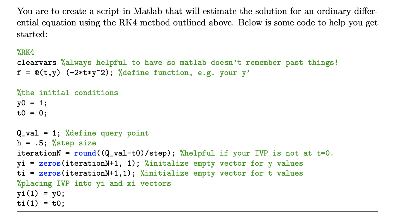
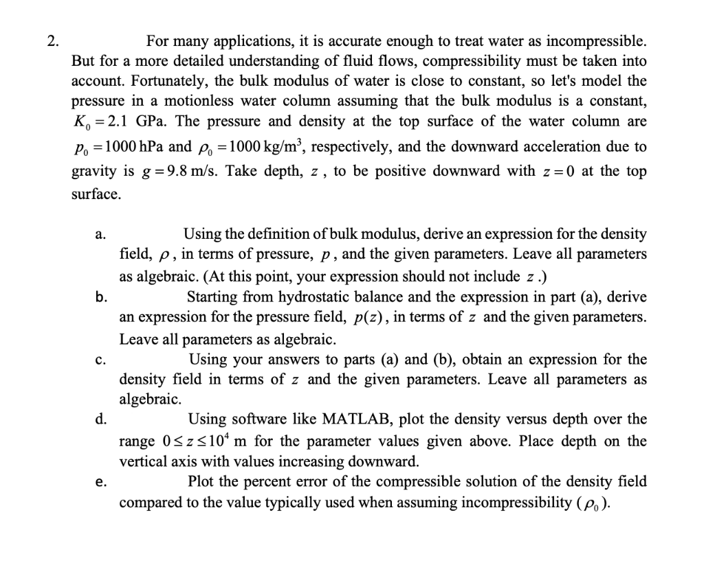
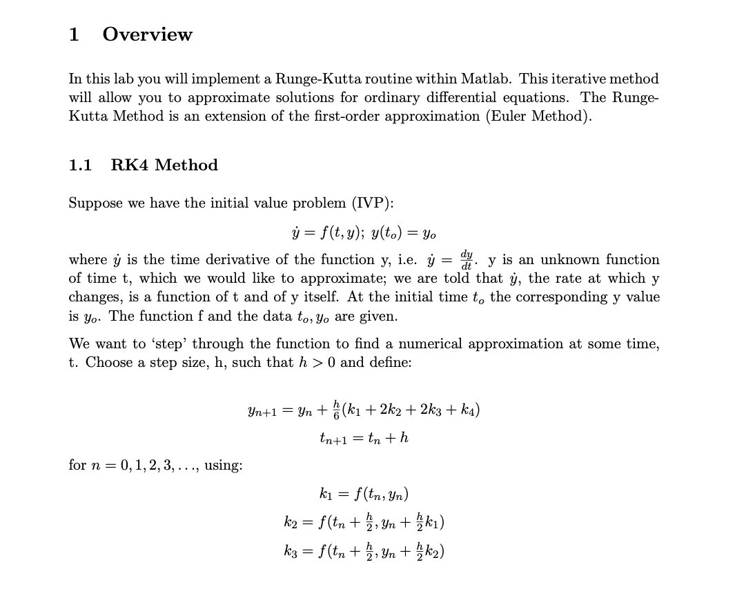
You are to create a script in Matlab that will estimate the solution for an ordinary differ- ential equation using the RK4 method outlined above. Below is some code to help you get started: %RK4 clearvars %always helpful to have so matlab doesn't remember past things! f = Q(t,y) (-2*t*y^2); %define function, e.g. your y = %the initial conditions yo 1; to = 0; = Q_val = 1; %define query point h = .5; %step size iterationN = round ((Q_val-t0)/step); %helpful if your IVP is not at t=0. yi = zeros(iterationN+1, 1); %initalize empty vector for y values ti = zeros(iterationN+1,1); %initialize empty vector for t values %placing IVP into yi and xi vectors yi(1) = yo; ti(1) = t0; 2. For many applications, it is accurate enough to treat water as incompressible. But for a more detailed understanding of fluid flows, compressibility must be taken into account. Fortunately, the bulk modulus of water is close to constant, so let's model the pressure in a motionless water column assuming that the bulk modulus is a constant, K. = 2.1 GPa. The pressure and density at the top surface of the water column are P. = 1000 hPa and p. =1000 kg/m, respectively, and the downward acceleration due to gravity is g =9.8 m/s. Take depth, z, to be positive downward with z = 0 at the top surface. a. b. an c. Using the definition of bulk modulus, derive an expression for the density field, p, in terms of pressure, p, and the given parameters. Leave all parameters as algebraic. (At this point, your expression should not include z.) Starting from hydrostatic balance and the expression in part (a), derive xpression for the pressure field, p(z), in terms of z and the given parameters. Leave all parameters as algebraic. Using your answers to parts (a) and (b), obtain an expression for the density field in terms of z and the given parameters. Leave all parameters as algebraic. Using software like MATLAB, plot the density versus depth over the range 05 z 5104 m for the parameter values given above. Place depth on the vertical axis with values increasing downward. Plot the percent error of the compressible solution of the density field compared to the value typically used when assuming incompressibility (p.). d. e. 1 Overview In this lab you will implement a Runge-Kutta routine within Matlab. This iterative method will allow you to approximate solutions for ordinary differential equations. The Runge- Kutta Method is an extension of the first-order approximation (Euler Method). 1.1 RK4 Method = Suppose we have the initial value problem (IVP): y = f(t, y); y(to) = yo where y is the time derivative of the function y, i.e. j = il y is an unknown function of time t, which we would like to approximate; we are told that y, the rate at which y changes, is a function of t and of y itself. At the initial time to the corresponding y value is yo. The function f and the data to, Yo are given. We want to 'step' through the function to find a numerical approximation at some time, t. Choose a step size, h, such that h> 0 and define: Yn+1 = yn + @ (ki + 2k2 + 2k3 + ka) tn+1=tn+h for n = 0,1,2,3,..., using: ki = f(tn, yn) k2 = f(tn + , Yn + Yn + ki) k3 = f(tn + , yn + ' k2) = =