

Answered step by step
Verified Expert Solution
Question
1 Approved Answer
Please use Simulink block diagram (MATLAB). EDIT: Below is what function you can use, and also how the block diagram may look like Question Two
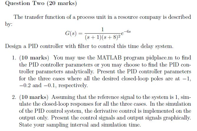
Please use Simulink block diagram (MATLAB). EDIT: Below is what function you can use, and also how the block diagram may look like 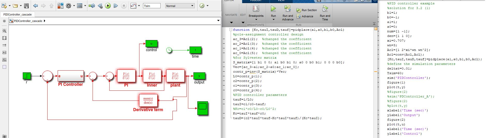
Step by Step Solution
There are 3 Steps involved in it
Step: 1

Get Instant Access to Expert-Tailored Solutions
See step-by-step solutions with expert insights and AI powered tools for academic success
Step: 2

Step: 3
Ace Your Homework with AI
Get the answers you need in no time with our AI-driven, step-by-step assistance
Get Started
Coping With Financial Accounting 1 For Senior Secondary Schools And Undergraduate Studies
Authors: Festus Chukwunwendu Akpotohwo ,Stella Alfred-Jaja Wellington-Igonibo ,Cletus Ogeibiri
1st Edition
3659611034, 978-3659611032