Please use stata and use answer part A and B and all part. Please be detailed in explanation.

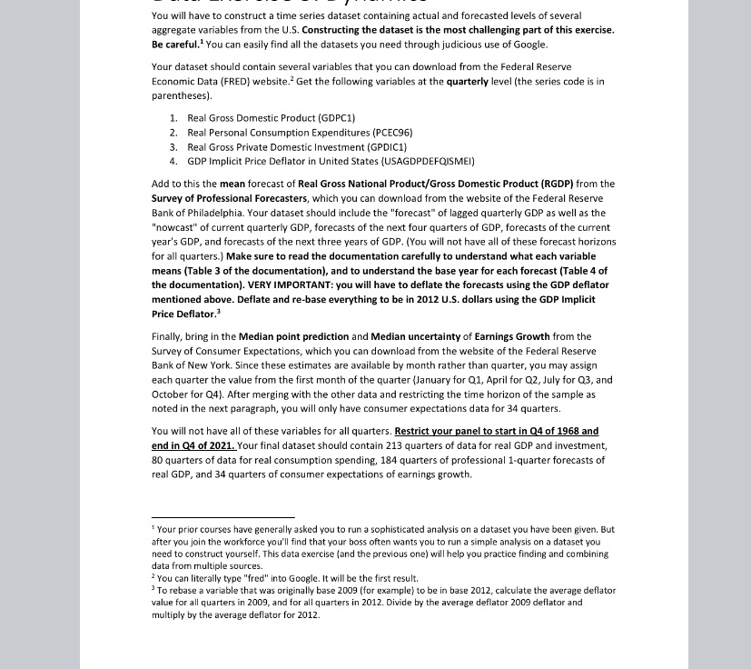
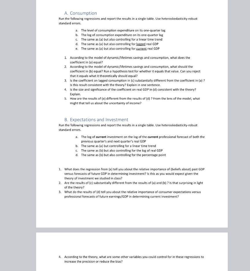
You will have to construct a time series dataset containing actual and forecasted levels of several aggregate variables from the U.5. Constructing the dataset is the most challenging part of this exercise. Be careful.' You can easily find all the datasets you need through judicious use of Google. Your dataset should contain several variables that you can download from the Federal Reserve Economic Data (FRED) website.' Get the following variables at the quarterly level (the series code is in parentheses). 1. Real Gross Domestic Product (GDPC1) 2. Real Personal Consumption Expenditures (PCEC96) 3. Real Gross Private Domestic Investment (GPDIC1) 4. GDP Implicit Price Deflator in United States (USAGDPDEFOISMEI) Add to this the mean forecast of Real Gross National Product/Gross Domestic Product (RGDP) from the Survey of Professional Forecasters, which you can download from the website of the Federal Reserve Bank of Philadelphia. Your dataset should include the "forecast" of lagged quarterly GDP as well as the "nowcast" of current quarterly GDP, forecasts of the next four quarters of GDP, forecasts of the current year's GDP, and forecasts of the next three years of GDP. (You will not have all of these forecast horizons for all quarters.) Make sure to read the documentation carefully to understand what each variable means (Table 3 of the documentation), and to understand the base year for each forecast (Table 4 of the documentation). VERY IMPORTANT: you will have to deflate the forecasts using the GDP deflator mentioned above. Deflate and re-base everything to be in 2012 U.S. dollars using the GDP Implicit Price Deflator.3 Finally, bring in the Median point prediction and Median uncertainty of Earnings Growth from the Survey of Consumer Expectations, which you can download from the website of the Federal Reserve Bank of New York. Since these estimates are available by month rather than quarter, you may assign each quarter the value from the first month of the quarter (January for Q1, April for Q2, July for Q3, and October for Q4). After merging with the other data and restricting the time horizon of the sample as noted in the next paragraph, you will only have consumer expectations data for 34 quarters. You will not have all of these variables for all quarters. Restrict your panel to start in 04 of 1968 and end in Q4 of 2021. Your final dataset should contain 213 quarters of data for real GDP and investment, 30 quarters of data for real consumption spending, 184 quarters of professional 1-quarter forecasts of real GDP, and 34 quarters of consumer expectations of earnings growth. Your prior courses have generally asked you to run a sophisticated analysis on a dataset you have been given. But after you join the workforce you'll find that your boss often wants you to run a simple analysis on a dataset you need to construct yourself. This data exercise (and the previous one) will help you practice finding and combining data from multiple sources. You can literally type "fred" into Google. It will be the first result. To rebase a variable that was originally base 2009 (for example) to be in base 2012, calculate the average deflator value for all quarters in 2009, and for all quarters in 2012. Divide by the average deflator 2009 deflator and multiply by the average deflator for 2012.A. Consumption Run the following regressions and report the results in a single table. Use heteroskedasticity-robust standard errors. a. The level of consumption expenditure on its one-quarter lag b. The log of consumption expenditure on its one-quarter lag c. The same as (a) but also controlling for a linear time trend d. The same as (a) but also controlling for lagged real GDP The same as (a) but also controlling for current real GDP 1. According to the model of dynamic/lifetimes savings and consumption, what does the coefficient in (a) equal 2. According to the model of dynamic/lifetimes savings and consumption, what should the coefficient in (b) equal? Run a hypothesis test for whether it equals that value. Can you reject that it equals what it theoretically should equal? 3. Is the coefficient on lagged consumption in (c) substantially different from the coefficient in (a) ? Is this result consistent with the theory? Explain in one sentence. 4. Is the size and significance of the coefficient on real GDP in (d) consistent with the theory? Explain. How are the results of (e) different from the results of (d) ? From the lens of the model, what might that tell us about the uncertainty of income? B. Expectations and Investment Run the following regressions and report the results in a single table. Use heteroskedasticity-robust standard errors. a. The log of current investment on the log of the current professional forecast of both the previous quarter's and next quarter's real GDP b. The same as (a) but controlling for a linear time trend C. The same as (b) but also controlling for the log of real GDP d. The same as (b) but also controlling for the percentage point 1. What does the regression from (a) tell you about the relative importance of (beliefs about) past GDP versus forecasts of future GDP in determining investment? Is this as you would expect given the theory of investment we studied in class? 2. Are the results of (c) substantially different from the results of (a) and (b) ? Is that surprising in light of the theory? 3. What do the results of (d) tell you about the relative importance of consumer expectations versus professional forecasts of future earnings/GDP in determining current investment? 4. According to the theory, what are some other variables you could control for in these regressions to increase the precision or reduce the bias?A. Consumption Run the following regressions and report the results in a single table. Use heteroskedasticity-robust standard errors. a. The level of consumption expenditure on its one-quarter lag b. The log of consumption expenditure on its one-quarter lag c. The same as (a) but also controlling for a linear time trend d. The same as (a) but also controlling for lagged real GDP The same as (a) but also controlling for current real GDP 1. According to the model of dynamic/lifetimes savings and consumption, what does the coefficient in (a) equal 2. According to the model of dynamic/lifetimes savings and consumption, what should the coefficient in (b) equal? Run a hypothesis test for whether it equals that value. Can you reject that it equals what it theoretically should equal? 3. Is the coefficient on lagged consumption in (c) substantially different from the coefficient in (a) ? Is this result consistent with the theory? Explain in one sentence. 4. Is the size and significance of the coefficient on real GDP in (d) consistent with the theory? Explain. How are the results of (e) different from the results of (d) ? From the lens of the model, what might that tell us about the uncertainty of income? B. Expectations and Investment Run the following regressions and report the results in a single table. Use heteroskedasticity-robust standard errors. a. The log of current investment on the log of the current professional forecast of both the previous quarter's and next quarter's real GDP b. The same as (a) but controlling for a linear time trend C. The same as (b) but also controlling for the log of real GDP d. The same as (b) but also controlling for the percentage point 1. What does the regression from (a) tell you about the relative importance of (beliefs about) past GDP versus forecasts of future GDP in determining investment? Is this as you would expect given the theory of investment we studied in class? 2. Are the results of (c) substantially different from the results of (a) and (b) ? Is that surprising in light of the theory? 3. What do the results of (d) tell you about the relative importance of consumer expectations versus professional forecasts of future earnings/GDP in determining current investment? 4. According to the theory, what are some other variables you could control for in these regressions to increase the precision or reduce the bias