Answered step by step
Verified Expert Solution
Link Copied!

Question

1 Approved Answer

please walk me through steps 8-13 8. Lindsey wants to determine how the sales of each month contributed to the total sales. Calculate this information

please walk me through steps 8-13 image text in transcribed
8. Lindsey wants to determine how the sales of each month contributed to the total sales. Calculate this information for her as follows: a. In cell B13, insert a formula without using a function that divides the total sales for January (cell B10) by the total sales to date (cell I10). b. Use an absolute reference to cell 110 in the formula. c. Use the Fill Handle to fill the range C13:G13 with the formula in cell B13. 9. Lindsey also needs to calculate the dividends earned each month. If the company earns $200,000 or more in a month, the dividend is 35% of the sales. If the company earns less than $200,000 in a month, the dividend is 27% of the sales. Calculate the dividends as follows: a. In cell B17, enter a formula that uses the IF function and tests whether the total sales for January (cell B10) is greater than or equal to 200000. b. If the condition is true, multiply the total sales for January (cell B10 ) by 0.35 to calculate a dividend of 35%. c. If the condition is false, multiply the total sales for January (cell B10) by 0.27 to calculate a dividend of 27%. d. Use the Fill Handle to fill the range C17:G17 with the formula in cell B17 to calculate the dividends for February through June. 10. Change the sparklines in the range H17:H18 as follows to use a more meaningful format: a. Change the Column sparklines to Line sparklines. b. Apply the sparkline style Dark Gray, Sparkline Style Dark \#3 (3rd column, 5 th row of the Sparkline Styles palette) to make the sparklines easier to see. 11. Lindsey would like to increase the average number of placements per month. Because executive placements are the most profitable, Lindsey wants to know how many executive placements she needs to reach the goal of 30 placements per month. Use Goal Seek to set the average number of placements for all positions (cell I27) to the value of 30 by changing the average number of executive placements (cell I23). 12. Format the text in cell 322 to clarify what it refers to as follows: a. Merge and center the range J22:327. b. Rotate the text down to 90 degrees in the merged cell so that the text reads from top to bottom. c. Change the width of column J to 6.00. 13. Delete row 35 , which contains information Lindsey does not need anymore

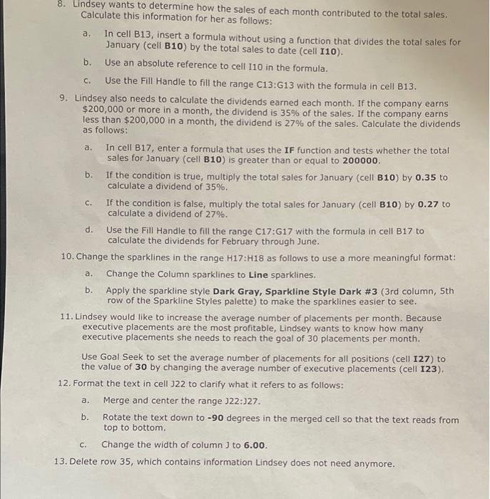
Step by Step Solution

There are 3 Steps involved in it

Step: 1

blur-text-image

Get Instant Access to Expert-Tailored Solutions

See step-by-step solutions with expert insights and AI powered tools for academic success

Step: 2

blur-text-image

Step: 3

blur-text-image

Ace Your Homework with AI

Get the answers you need in no time with our AI-driven, step-by-step assistance

Get Started

Recommended Textbook for

Database Design Application And Administration

Authors: Michael Mannino, Michael V. Mannino

2nd Edition

0072880678, 9780072880670

More Books

Students also viewed these Databases questions

Question

Find dy/dx if x = te, y = 2t2 +1

Answered: 1 week ago