PLEASE WRITE MATLAB CODE AND INCLUDE ALL PLOTS


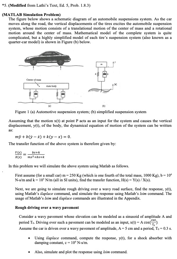
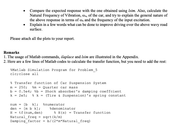
*5. (Modified from Lathi's Text, Ed. 5, Prob. 1.8.3) (MATLAB Simulation Problem) The figure below shows a schematic diagram of an automobile suspensions system. As the car moves along the road, the vertical displacements of the tires excites the automobile suspension system, whose motion consists of a translational motion of the center of mass and a rotational motion around the center of mass. Mathematical model of the complete system is quite complicated, but a highly simplified model of each tire's suspension system (also known as a quarter-car model) is shown in Figure (b) below. Center of mass Auto body (6) Figure 1 (a) Automotive suspension system; (b) simplified suspension system Assuming that the motion x(t) at point P acts as an input for the system and causes the vertical displacement, y(t), of the body, the dynamical equation of motion of the system can be written as: my + b- *)+k(y - x) = 0. The transfer function of the above system is therefore given by: Y(S) - x(s) bs+k ms2+bs+k In this problem we will simulate the above system using Matlab as follows. First assume (for a small car) m=250 Kg (which is one fourth of the total mass, 1000 Kg), b= 104 N-s/m and k = 10 N/m (all in SI units), find the transfer function, H(s) = Y(S) /X(). Next, we are going to simulate rough driving over a wavy road surface, find the response, y(t), using Matlab's ilaplace command, and simulate the response using Matlab's Isim command. The usage of Matlab's Isim and ilaplace commands are illustrated in the Appendix. Rough driving over a wavy pavement Consider a wavy pavement whose elevation can be modeled as a sinusoid of amplitude A and period To. Driving over such a pavement can be modeled as an input, x(t) = A cos ). Assume the car is driven over a wavy pavement of amplitude, A= 5 cm and a period, To = 0.3 s. Using ilaplace command, compute the response, y(t), for a shock absorber with damping constant, c = 10N-s/m. . Also, simulate and plot the response using Isim command. Compare the expected response with the one obtained using lsim. Also, calculate the Natural Frequency of Vibration, On, of the car, and try to explain the general nature of the above response in terms of o, and the frequency of the input excitation. Explain in a few words what can be done to improve driving over the above wavy road surface. Please attach all the plots to your report. Remarks 1. The usage of Matlab commands, ilaplace and Isim are illustrated in the Appendix. 2. Here are a few lines of Matlab codes to calculate the transfer function, but you need to add the rest: #Matlab Simulation Program for Problem_5 clc;close all & Transfer function of Car Suspension System m = 250; fm = Quarter car mass b = 0.5e4; b = Shock absorber's damping coeffcient k = 2e5; $k = (Tire & Suspension)'s spring constant num = (b k); $numerator den = ( mbk]; denominator H = tf (num, den) H(s) = Transfer function Natural freq = sqrt (k/m) Damping_factor = b/(2*m*Natural_freq) *5. (Modified from Lathi's Text, Ed. 5, Prob. 1.8.3) (MATLAB Simulation Problem) The figure below shows a schematic diagram of an automobile suspensions system. As the car moves along the road, the vertical displacements of the tires excites the automobile suspension system, whose motion consists of a translational motion of the center of mass and a rotational motion around the center of mass. Mathematical model of the complete system is quite complicated, but a highly simplified model of each tire's suspension system (also known as a quarter-car model) is shown in Figure (b) below. Center of mass Auto body (6) Figure 1 (a) Automotive suspension system; (b) simplified suspension system Assuming that the motion x(t) at point P acts as an input for the system and causes the vertical displacement, y(t), of the body, the dynamical equation of motion of the system can be written as: my + b- *)+k(y - x) = 0. The transfer function of the above system is therefore given by: Y(S) - x(s) bs+k ms2+bs+k In this problem we will simulate the above system using Matlab as follows. First assume (for a small car) m=250 Kg (which is one fourth of the total mass, 1000 Kg), b= 104 N-s/m and k = 10 N/m (all in SI units), find the transfer function, H(s) = Y(S) /X(). Next, we are going to simulate rough driving over a wavy road surface, find the response, y(t), using Matlab's ilaplace command, and simulate the response using Matlab's Isim command. The usage of Matlab's Isim and ilaplace commands are illustrated in the Appendix. Rough driving over a wavy pavement Consider a wavy pavement whose elevation can be modeled as a sinusoid of amplitude A and period To. Driving over such a pavement can be modeled as an input, x(t) = A cos ). Assume the car is driven over a wavy pavement of amplitude, A= 5 cm and a period, To = 0.3 s. Using ilaplace command, compute the response, y(t), for a shock absorber with damping constant, c = 10N-s/m. . Also, simulate and plot the response using Isim command. Compare the expected response with the one obtained using lsim. Also, calculate the Natural Frequency of Vibration, On, of the car, and try to explain the general nature of the above response in terms of o, and the frequency of the input excitation. Explain in a few words what can be done to improve driving over the above wavy road surface. Please attach all the plots to your report. Remarks 1. The usage of Matlab commands, ilaplace and Isim are illustrated in the Appendix. 2. Here are a few lines of Matlab codes to calculate the transfer function, but you need to add the rest: #Matlab Simulation Program for Problem_5 clc;close all & Transfer function of Car Suspension System m = 250; fm = Quarter car mass b = 0.5e4; b = Shock absorber's damping coeffcient k = 2e5; $k = (Tire & Suspension)'s spring constant num = (b k); $numerator den = ( mbk]; denominator H = tf (num, den) H(s) = Transfer function Natural freq = sqrt (k/m) Damping_factor = b/(2*m*Natural_freq)


