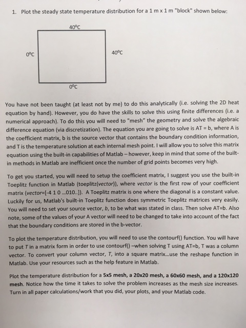
Plot the steady state temp distribution for a 1x1 m block shown below:

Plot the steady state temperature distribution for a 1 m times 1 m "block" shown below: You have not been taught (at least not by me) to do this analytically (i.e. solving the 20 heat equation by hand). However, you do have the skills to solve this using finite differences (i.e. a numerical approach). To do this you will need to "mesh" the geometry and solve the algebraic difference equation (via). The equation you are going to solve is AT = b, where A is the coefficient matrix, b is the source vector that contains the boundary condition information, and T is the temperature solution at each internal mesh point. I will allow you to solve this matrix equation using the built-in capabilities of Matlab - however, keep in mind that some of the built-in methods in Matlab are inefficient once the number of grid points becomes very high. To get you started, you will need to setup the coefficient matrix, I suggest you use the built-in function in, where vector is the first row of your coefficient matrix (vector = [-4 1 0 ...010..]). A matrix is one where the diagonal is a constant value. Luckily for us, Matlab's built-in function does symmetric matrices very easily. You will need to set your source vector, b. to be what was stated in class. Then solve AT=b. Also note, some of the values of your A vector will need to be changed to take into account of the fact that the boundary conditions are stored in the b-vector. To plot the temperature distribution, you will need to use the contourf() function. You will have to put T in a matrix form in order to use contourf() -when solving T using AT=b, T was a column vector. To convert your column vector, T, into a square matrix...use the reshape function in Matlab. Use your resources such as the help feature in Matlab. Plot the temperature distribution for a 5 times 5 mesh, a 20 times 20 mesh, a 60 times 60 mesh, and a 120 times 120 mesh. Notice how the time it takes to solve the problem increases as the mesh size increases. Turn in all paper calculations/work that you did, your plots, and your Matlab code. Plot the steady state temperature distribution for a 1 m times 1 m "block" shown below: You have not been taught (at least not by me) to do this analytically (i.e. solving the 20 heat equation by hand). However, you do have the skills to solve this using finite differences (i.e. a numerical approach). To do this you will need to "mesh" the geometry and solve the algebraic difference equation (via). The equation you are going to solve is AT = b, where A is the coefficient matrix, b is the source vector that contains the boundary condition information, and T is the temperature solution at each internal mesh point. I will allow you to solve this matrix equation using the built-in capabilities of Matlab - however, keep in mind that some of the built-in methods in Matlab are inefficient once the number of grid points becomes very high. To get you started, you will need to setup the coefficient matrix, I suggest you use the built-in function in, where vector is the first row of your coefficient matrix (vector = [-4 1 0 ...010..]). A matrix is one where the diagonal is a constant value. Luckily for us, Matlab's built-in function does symmetric matrices very easily. You will need to set your source vector, b. to be what was stated in class. Then solve AT=b. Also note, some of the values of your A vector will need to be changed to take into account of the fact that the boundary conditions are stored in the b-vector. To plot the temperature distribution, you will need to use the contourf() function. You will have to put T in a matrix form in order to use contourf() -when solving T using AT=b, T was a column vector. To convert your column vector, T, into a square matrix...use the reshape function in Matlab. Use your resources such as the help feature in Matlab. Plot the temperature distribution for a 5 times 5 mesh, a 20 times 20 mesh, a 60 times 60 mesh, and a 120 times 120 mesh. Notice how the time it takes to solve the problem increases as the mesh size increases. Turn in all paper calculations/work that you did, your plots, and your Matlab code


