pls help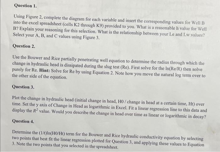

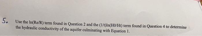
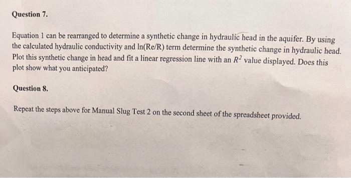
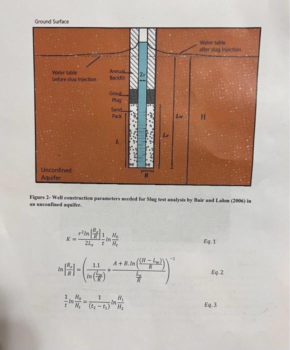
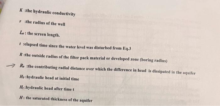
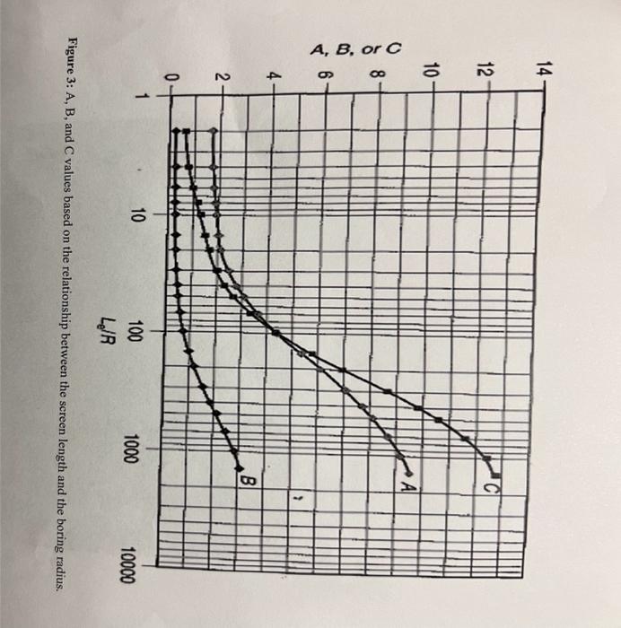
Using Figure 2, complete the diagram for each variable and insert the corresponding values for Well B into the excel spreadsheet (cells K2 through K9) provided to you. What is a reasonable h value for Well B? Explain your reasoning for this selection. What is the relationship between your Le and Lw values? Select your A, B, and C values using Figure 3 . Question 2. Use the Bouwer and Rice partially penetrating well equation to determine the radius through which the change in hydraulic head is dissipated during the slug test (Re). First solve for the ln(Re/R) then solve purely for Re. Hint: Solve for Re by using Equation 2. Note how you move the natural log term over to the other side of the equation. Question 3. Plot the change in hydraulic head (initial change in head, H0 / change in head at a certain time, Ht) over time. Set the y axis of Change in Head as logarithmic in Excel. Fit a linear regression line to this data and display the R2 value. Would you describe the change in head over time as linear or logarithmic in decay? Question 4. Determine the (1/t)ln(H/Ht) term for the Bouwer and Rice hydraulic conductivity equation by selecting two points that best fit the linear regression plotted for Question 3, and applying these values to Equation 3. Note the two points that you selected in the spreadsheet. Use the ln(Re/R) term found in Question 2 and the (1/t)ln(H0/Ht) term found in Question 4 to determine the hydraulic conductivity of the aquifer culminating with Equation 1. Equation 1 can be rearranged to determine a synthetic change in hydraulic head in the aquifer. By using the calculated hydraulic conductivity and ln(Re/R) term determine the synthetic change in hydraulic head. Plot this synthetic change in head and fit a linear regression line with an R2 value displayed. Does this plot show what you anticipated? Question 8. Repeat the steps above for Manual Slug Test 2 on the second sheet of the spreadsheet provided. As we have learned, performing a slug test can help determine important properties from an aquifer. During this lab we will go over the slug test data recorded in the field trip to the River Barge Park. We will analyze the data recorded manually for well A and B. Figure 1 - Aerial imagery from the River Barge Park with the studied wells Methods River Barge Park is located on unconsolidated, heterogeneous sediments with a total of 7 wells installed in the study area. Two manual slug tests were performed at the central-most well, Well B, shown in Figure 1. Well B is 15 feet in length, has a nuduius of 2 inches, has a boring fudius of 4 inches, and is screened all the way to the top of the casing. To process this data to the fullest extent, it is necessary to use the Bouwer and Rice Method to determine the hydraulic conductivity of the unconfined aquifer beneath River Barge Park. The Bouwer and Rice Method works for partially penetrating wells and is therefore more versatile - it will be the objective of today's practical to learn and apply this method. Figure 2- Well construction parameters needed for Slug test analysis by Bair and Lahm (2006) in an unconfined aquifer. K=2Ler2ln[RRe]t1lnHtH0 Eq. 1 ln[RRe]=(ln(RLw)1.1+RLeA+Bln(R(HLw)))1 Eq.2 t1lnHtH0=(t2t1)1lnH2H1 Eq.3 K :the hydraulic conductivity r :the radius of the well Le : the screen length. t :elapsed time since the water level was disturbed from Eq.3 R :the outside radius of the filter pack material or developed zone (boring radius) Re :the contributing radial distance over which the difference in head is dissipated in the aquifer H0:hydraulic head at initial time Ht :hydraulic head after time t H : the saturated thickness of the aquifer Using Figure 2, complete the diagram for each variable and insert the corresponding values for Well B into the excel spreadsheet (cells K2 through K9) provided to you. What is a reasonable h value for Well B? Explain your reasoning for this selection. What is the relationship between your Le and Lw values? Select your A, B, and C values using Figure 3 . Question 2. Use the Bouwer and Rice partially penetrating well equation to determine the radius through which the change in hydraulic head is dissipated during the slug test (Re). First solve for the ln(Re/R) then solve purely for Re. Hint: Solve for Re by using Equation 2. Note how you move the natural log term over to the other side of the equation. Question 3. Plot the change in hydraulic head (initial change in head, H0 / change in head at a certain time, Ht) over time. Set the y axis of Change in Head as logarithmic in Excel. Fit a linear regression line to this data and display the R2 value. Would you describe the change in head over time as linear or logarithmic in decay? Question 4. Determine the (1/t)ln(H/Ht) term for the Bouwer and Rice hydraulic conductivity equation by selecting two points that best fit the linear regression plotted for Question 3, and applying these values to Equation 3. Note the two points that you selected in the spreadsheet. Use the ln(Re/R) term found in Question 2 and the (1/t)ln(H0/Ht) term found in Question 4 to determine the hydraulic conductivity of the aquifer culminating with Equation 1. Equation 1 can be rearranged to determine a synthetic change in hydraulic head in the aquifer. By using the calculated hydraulic conductivity and ln(Re/R) term determine the synthetic change in hydraulic head. Plot this synthetic change in head and fit a linear regression line with an R2 value displayed. Does this plot show what you anticipated? Question 8. Repeat the steps above for Manual Slug Test 2 on the second sheet of the spreadsheet provided. As we have learned, performing a slug test can help determine important properties from an aquifer. During this lab we will go over the slug test data recorded in the field trip to the River Barge Park. We will analyze the data recorded manually for well A and B. Figure 1 - Aerial imagery from the River Barge Park with the studied wells Methods River Barge Park is located on unconsolidated, heterogeneous sediments with a total of 7 wells installed in the study area. Two manual slug tests were performed at the central-most well, Well B, shown in Figure 1. Well B is 15 feet in length, has a nuduius of 2 inches, has a boring fudius of 4 inches, and is screened all the way to the top of the casing. To process this data to the fullest extent, it is necessary to use the Bouwer and Rice Method to determine the hydraulic conductivity of the unconfined aquifer beneath River Barge Park. The Bouwer and Rice Method works for partially penetrating wells and is therefore more versatile - it will be the objective of today's practical to learn and apply this method. Figure 2- Well construction parameters needed for Slug test analysis by Bair and Lahm (2006) in an unconfined aquifer. K=2Ler2ln[RRe]t1lnHtH0 Eq. 1 ln[RRe]=(ln(RLw)1.1+RLeA+Bln(R(HLw)))1 Eq.2 t1lnHtH0=(t2t1)1lnH2H1 Eq.3 K :the hydraulic conductivity r :the radius of the well Le : the screen length. t :elapsed time since the water level was disturbed from Eq.3 R :the outside radius of the filter pack material or developed zone (boring radius) Re :the contributing radial distance over which the difference in head is dissipated in the aquifer H0:hydraulic head at initial time Ht :hydraulic head after time t H : the saturated thickness of the aquifer