Portfolio optimization with N risky assets

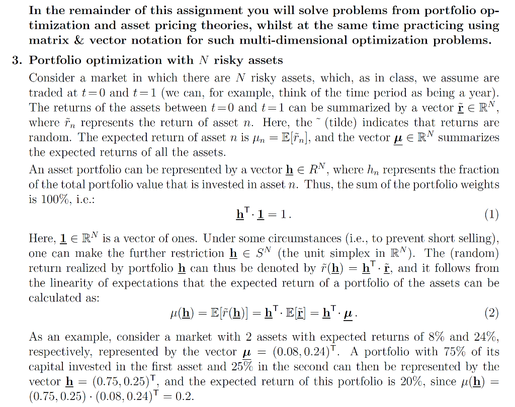
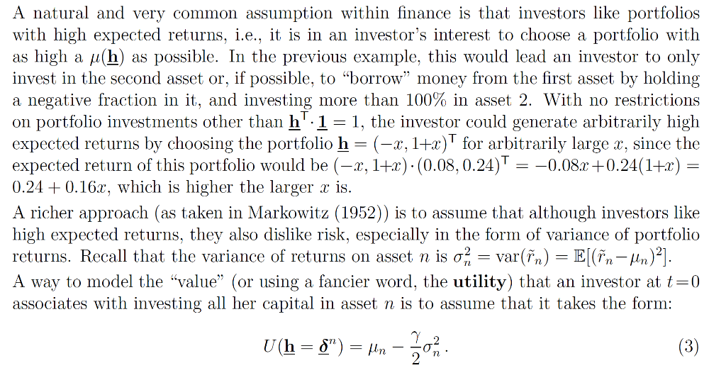
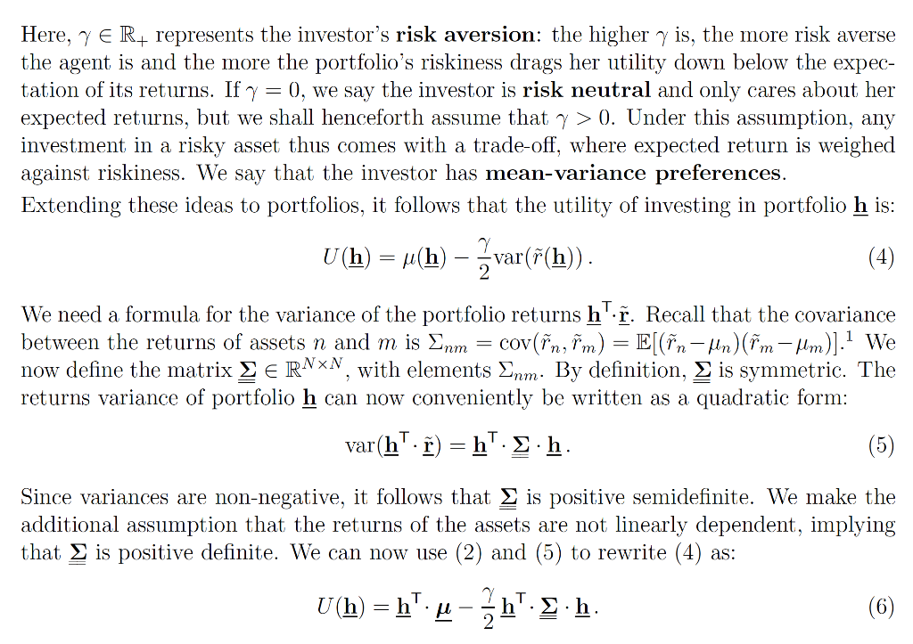
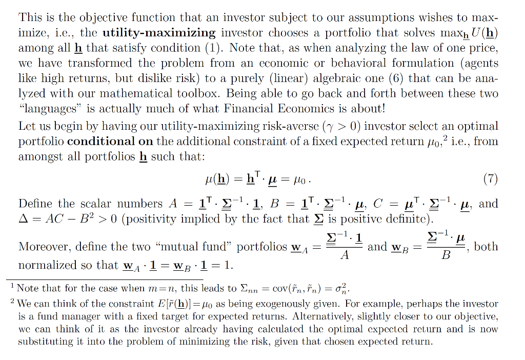
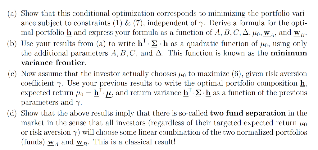
In the remainder of this assignment you will solve problems from portfolio op- timization and asset pricing theories, whilst at the same time practicing using matrix & vector notation for such multi-dimensional optimization problems. 3. Portfolio optimization with N risky assets Consider a market in which there are N risky assets, which, as in class, we assume are traded at t=0 and t=1 (we can, for example, think of the time period as being a year). The returns of the assets between t=0 and t=1 can be summarized by a vector r ERN, where in represents the return of asset n. Here, the (tilde) indicates that returns are random. The expected return of asset n is hin = E[in], and the vector u ERN summarizes the expected returns of all the assets. An asset portfolio can be represented by a vector h ER, where hn represents the fraction of the total portfolio value that is invested in asset n. Thus, the sum of the portfolio weights is 100%, i.e.: h":1=1. (1) Here, 1 ERM is a vector of ones. Under some circumstances (i.e., to prevent short selling), one can make the further restriction h ESN (the unit simplex in R^). The (random) return realized by portfolio h can thus be denoted by r(h) = h'. , and it follows from the linearity of expectations that the expected return of a portfolio of the assets can be calculated as: u(h) = E[F(h)] = h'. Et = h'.d. As an example, consider a market with 2 assets with expected returns of 8% and 24%, respectively, represented by the vector u = (0.08, 0.24)". A portfolio with 75% of its capital invested in the first asset and 25% in the second can then be represented by the vector h = (0.75, 0.25)', and the expected return of this portfolio is 20%, since u(h) = (0.75, 0.25) (0.08,0.24) = 0.2. (2) A natural and very common assumption within finance is that investors like portfolios with high expected returns, i.e., it is in an investor's interest to choose a portfolio with as high a uch as possible. In the previous example, this would lead an investor to only invest in the second asset or, if possible, to "borrow" money from the first asset by holding a negative fraction in it, and investing more than 100% in asset 2. With no restrictions on portfolio investments other than h'.1=1, the investor could generate arbitrarily high expected returns by choosing the portfolio h= (-x, 1+x) for arbitrarily large x, since the expected return of this portfolio would be (-2, 1+.x)(0.08, 0.24)T = -0.08.2 +0.24(1+x) = 0.24 + 0.16x, which is higher the larger x is. A richer approach (as taken in Markowitz (1952)) is to assume that although investors like high expected returns, they also dislike risk, especially in the form of variance of portfolio returns. Recall that the variance of returns on asset n is 07 = var(in) = E[(in-Mn)?]. A way to model the "value (or using a fancier word, the utility) that an investor at t=0 associates with investing all her capital in asset n is to assume that it takes the form: Uh = 8) = In - Sn (3) Here, y eR represents the investor's risk aversion: the higher y is, the more risk averse the agent is and the more the portfolio's riskiness drags her utility down below the expec- tation of its returns. If y = 0, we say the investor is risk neutral and only cares about her expected returns, but we shall henceforth assume that 7 > 0. Under this assumption, any investment in a risky asset thus comes with a trade-off, where expected return is weighed against riskiness. We say that the investor has mean-variance preferences. Extending these ideas to portfolios, it follows that the utility of investing in portfolio h is: U(h) = u(h) - var(F(h)). We need a formula for the variance of the portfolio returns h'.. Recall that the covariance between the returns of assets n and m is Enm = cov(in, m) = E[(in-Mn)(im-Mm)].1 We now define the matrix LERNXN, with elements Inm. By definition, is symmetric. The returns variance of portfolio h can now conveniently be written as a quadratic form: var(h". ) = h'...h. (5) Since variances are non-negative, it follows that is positive semidefinite. We make the additional assumption that the returns of the assets are not linearly dependent, implying that is positive definite. We can now use (2) and (5) to rewrite (4) as: U(h) = h'. 4-h..h. T (6) This is the objective function that an investor subject to our assumptions wishes to max- imize, i.e., the utility-maximizing investor chooses a portfolio that solves maxh U(h) among all h that satisfy condition (1). Note that, as when analyzing the law of one price, we have transformed the problem from an economic or behavioral formulation (agents like high returns, but dislike risk) to a purely (linear) algebraic one (6) that can be ana- lyzed with our mathematical toolbox. Being able to go back and forth between these two "languages" is actually much of what Financial Economics is about! Let us begin by having our utility-maximizing risk-averse (7 > 0) investor select an optimal portfolio conditional on the additional constraint of a fixed expected return po.? i.e., from amongst all portfolios h such that: u(h) = h' u = Ho. (7) Define the scalar numbers A = 1'.1-1.1, B = 1". -'., C = ut. S', and A= AC B2 > 0 (positivity implied by the fact that is positive definite). > 5-1 Moreover, define the two "mutual fund portfolios wa = and wp== F, both A normalized so that wa:1=WB:1=1. 1 1 Note that for the case when m=n, this leads to Enn = cov(in, in) = 02. 2 We can think of the constraint E[f(h)]=No as being exogenously given. For example, perhaps the investor is a fund manager with a fixed target for expected returns. Alternatively, slightly closer to our objective, we can think of it as the investor already having calculated the optimal expected return and is now substituting it into the problem of minimizing the risk, given that chosen expected return. a) Show that this conditional optimization corresponds to minimizing the portfolio vari- ance subject to constraints (1) & (7), independent of y. Derive a formula for the opti- mal portfolio h and express your formula as a function of A, B, C, A, HO, WA, and wh. (b) Use your results from (a) to write h...h as a quadratic function of No, using only the additional parameters A, B, C, and A. This function is known as the minimum variance frontier. Now assume that the investor actually chooses up to maximize (6), given risk aversion coefficient 7. Use your previous results to write the optimal portfolio composition h, expected return po = h'. u, and return variance h'..h as a function of the previous parameters and 7. Show that the above results imply that there is so-called two fund separation in the market in the sense that all investors (regardless of their targeted expected return po or risk aversion will choose some linear combination of the two normalized portfolios (funds) w, and WB. This is a classical result! In the remainder of this assignment you will solve problems from portfolio op- timization and asset pricing theories, whilst at the same time practicing using matrix & vector notation for such multi-dimensional optimization problems. 3. Portfolio optimization with N risky assets Consider a market in which there are N risky assets, which, as in class, we assume are traded at t=0 and t=1 (we can, for example, think of the time period as being a year). The returns of the assets between t=0 and t=1 can be summarized by a vector r ERN, where in represents the return of asset n. Here, the (tilde) indicates that returns are random. The expected return of asset n is hin = E[in], and the vector u ERN summarizes the expected returns of all the assets. An asset portfolio can be represented by a vector h ER, where hn represents the fraction of the total portfolio value that is invested in asset n. Thus, the sum of the portfolio weights is 100%, i.e.: h":1=1. (1) Here, 1 ERM is a vector of ones. Under some circumstances (i.e., to prevent short selling), one can make the further restriction h ESN (the unit simplex in R^). The (random) return realized by portfolio h can thus be denoted by r(h) = h'. , and it follows from the linearity of expectations that the expected return of a portfolio of the assets can be calculated as: u(h) = E[F(h)] = h'. Et = h'.d. As an example, consider a market with 2 assets with expected returns of 8% and 24%, respectively, represented by the vector u = (0.08, 0.24)". A portfolio with 75% of its capital invested in the first asset and 25% in the second can then be represented by the vector h = (0.75, 0.25)', and the expected return of this portfolio is 20%, since u(h) = (0.75, 0.25) (0.08,0.24) = 0.2. (2) A natural and very common assumption within finance is that investors like portfolios with high expected returns, i.e., it is in an investor's interest to choose a portfolio with as high a uch as possible. In the previous example, this would lead an investor to only invest in the second asset or, if possible, to "borrow" money from the first asset by holding a negative fraction in it, and investing more than 100% in asset 2. With no restrictions on portfolio investments other than h'.1=1, the investor could generate arbitrarily high expected returns by choosing the portfolio h= (-x, 1+x) for arbitrarily large x, since the expected return of this portfolio would be (-2, 1+.x)(0.08, 0.24)T = -0.08.2 +0.24(1+x) = 0.24 + 0.16x, which is higher the larger x is. A richer approach (as taken in Markowitz (1952)) is to assume that although investors like high expected returns, they also dislike risk, especially in the form of variance of portfolio returns. Recall that the variance of returns on asset n is 07 = var(in) = E[(in-Mn)?]. A way to model the "value (or using a fancier word, the utility) that an investor at t=0 associates with investing all her capital in asset n is to assume that it takes the form: Uh = 8) = In - Sn (3) Here, y eR represents the investor's risk aversion: the higher y is, the more risk averse the agent is and the more the portfolio's riskiness drags her utility down below the expec- tation of its returns. If y = 0, we say the investor is risk neutral and only cares about her expected returns, but we shall henceforth assume that 7 > 0. Under this assumption, any investment in a risky asset thus comes with a trade-off, where expected return is weighed against riskiness. We say that the investor has mean-variance preferences. Extending these ideas to portfolios, it follows that the utility of investing in portfolio h is: U(h) = u(h) - var(F(h)). We need a formula for the variance of the portfolio returns h'.. Recall that the covariance between the returns of assets n and m is Enm = cov(in, m) = E[(in-Mn)(im-Mm)].1 We now define the matrix LERNXN, with elements Inm. By definition, is symmetric. The returns variance of portfolio h can now conveniently be written as a quadratic form: var(h". ) = h'...h. (5) Since variances are non-negative, it follows that is positive semidefinite. We make the additional assumption that the returns of the assets are not linearly dependent, implying that is positive definite. We can now use (2) and (5) to rewrite (4) as: U(h) = h'. 4-h..h. T (6) This is the objective function that an investor subject to our assumptions wishes to max- imize, i.e., the utility-maximizing investor chooses a portfolio that solves maxh U(h) among all h that satisfy condition (1). Note that, as when analyzing the law of one price, we have transformed the problem from an economic or behavioral formulation (agents like high returns, but dislike risk) to a purely (linear) algebraic one (6) that can be ana- lyzed with our mathematical toolbox. Being able to go back and forth between these two "languages" is actually much of what Financial Economics is about! Let us begin by having our utility-maximizing risk-averse (7 > 0) investor select an optimal portfolio conditional on the additional constraint of a fixed expected return po.? i.e., from amongst all portfolios h such that: u(h) = h' u = Ho. (7) Define the scalar numbers A = 1'.1-1.1, B = 1". -'., C = ut. S', and A= AC B2 > 0 (positivity implied by the fact that is positive definite). > 5-1 Moreover, define the two "mutual fund portfolios wa = and wp== F, both A normalized so that wa:1=WB:1=1. 1 1 Note that for the case when m=n, this leads to Enn = cov(in, in) = 02. 2 We can think of the constraint E[f(h)]=No as being exogenously given. For example, perhaps the investor is a fund manager with a fixed target for expected returns. Alternatively, slightly closer to our objective, we can think of it as the investor already having calculated the optimal expected return and is now substituting it into the problem of minimizing the risk, given that chosen expected return. a) Show that this conditional optimization corresponds to minimizing the portfolio vari- ance subject to constraints (1) & (7), independent of y. Derive a formula for the opti- mal portfolio h and express your formula as a function of A, B, C, A, HO, WA, and wh. (b) Use your results from (a) to write h...h as a quadratic function of No, using only the additional parameters A, B, C, and A. This function is known as the minimum variance frontier. Now assume that the investor actually chooses up to maximize (6), given risk aversion coefficient 7. Use your previous results to write the optimal portfolio composition h, expected return po = h'. u, and return variance h'..h as a function of the previous parameters and 7. Show that the above results imply that there is so-called two fund separation in the market in the sense that all investors (regardless of their targeted expected return po or risk aversion will choose some linear combination of the two normalized portfolios (funds) w, and WB. This is a classical result