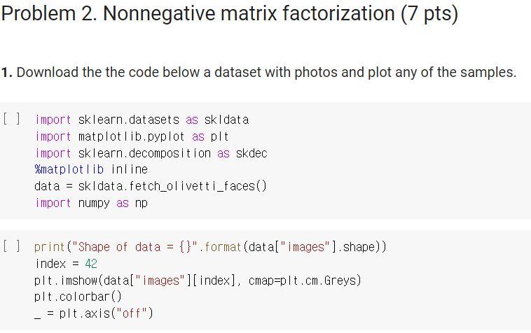
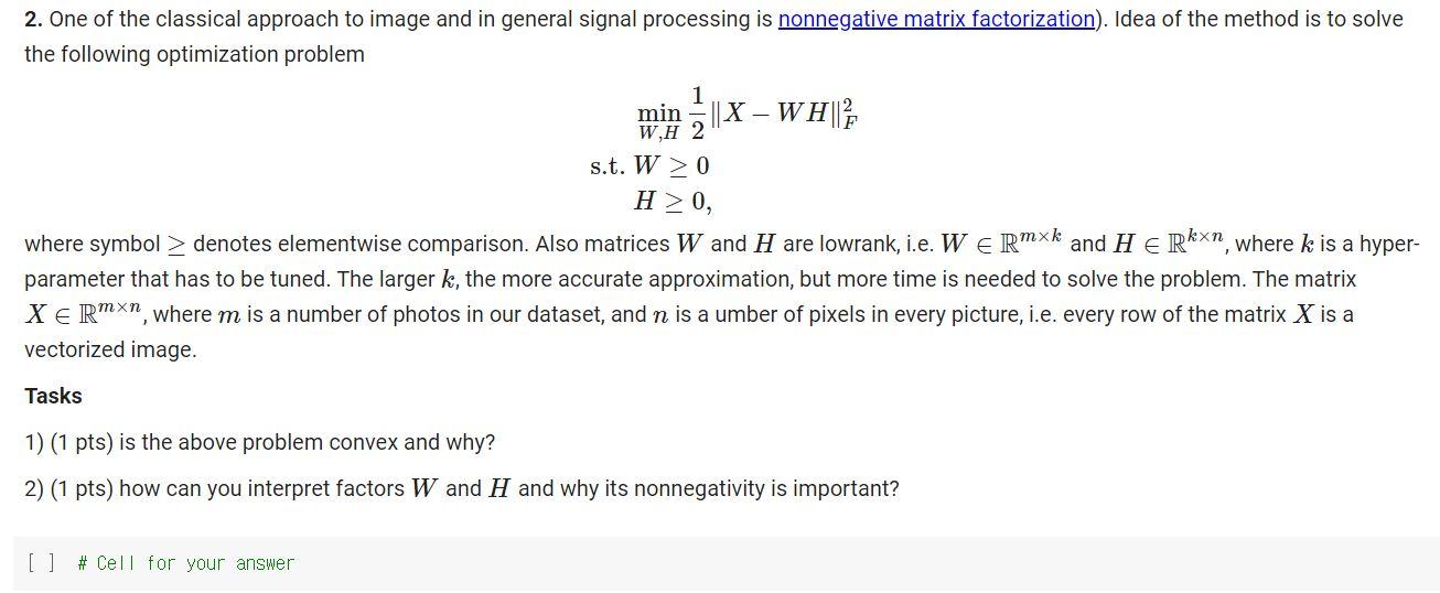
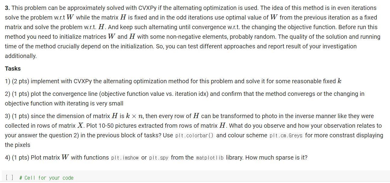
Problem 2. Nonnegative matrix factorization (7 pts) 1. Download the the code below a dataset with photos and plot any of the samples. [] import sklearn datasets as skidata import matplot lib.pyplot as plt import sklearn. decomposition as skdec %matplot lib inline data = skidata.fetch_olivetti_faces() import numpy as np = [] print("Shape of data = {}", format (data["images").shape)) index = 42 plt. imshow(data["images"][index]. cmap=plt.cm. Greys) plt.colorbar) _ = plt.axis("off") WH || 2. One of the classical approach to image and in general signal processing is nonnegative matrix factorization). Idea of the method is to solve the following optimization problem 1 min X WH 2 s.t. W > 0 H>0, where symbol > denotes elementwise comparison. Also matrices W and H are lowrank, i.e. W e Rmxk and H eRkxn, where k is a hyper- parameter that has to be tuned. The larger k, the more accurate approximation, but more time is needed to solve the problem. The matrix XE RMXn, where m is a number of photos in our dataset, and n is a umber of pixels in every picture, i.e. every row of the matrix X is a vectorized image. Tasks 1) (1 pts) is the above problem convex and why? 2) (1 pts) how can you interpret factors W and H and why its nonnegativity is important? [] # Cell for your answer 3. This problem can be approximately solved with CVXPy if the alternating optimization is used. The idea of this method is in even iterations solve the problem w.r.t W while the matrix H is fixed and in the odd iterations use optimal value of W from the previous iteration as a fixed matrix and solve the problem w.r.t. H. And keep such alternating until convergence w.r.t. the changing the objective function. Before run this method you need to initialize matrices W and H with some non-negative elements, probably random. The quality of the solution and running time of the method crucially depend on the initialization. So, you can test different approaches and report result of your investigation additionally. Tasks 1) (2 pts) implement with CVXPy the alternating optimization method for this problem and solve it for some reasonable fixed k 2) (1 pts) plot the convergence line (objective function value vs. iteration idx) and confirm that the method converegs or the changing in objective function with iterating is very small 3) (1 pts) since the dimension of matrix H is k x n, then every row of H can be transformed to photo in the inverse manner like they were collected in rows of matrix X. Plot 10-50 pictures extracted from rows of matrix H. What do you observe and how your observation relates to your answer the question 2) in the previous block of tasks? Use plt.colorbar() and colour scheme pit.cm. Greys for more constrast displaying the pixels 4) (1 pts) Plot matrix W with functions plt. imshow or plt.spy from the matplotlib library. How much sparse is it? [] # Cell for your code Problem 2. Nonnegative matrix factorization (7 pts) 1. Download the the code below a dataset with photos and plot any of the samples. [] import sklearn datasets as skidata import matplot lib.pyplot as plt import sklearn. decomposition as skdec %matplot lib inline data = skidata.fetch_olivetti_faces() import numpy as np = [] print("Shape of data = {}", format (data["images").shape)) index = 42 plt. imshow(data["images"][index]. cmap=plt.cm. Greys) plt.colorbar) _ = plt.axis("off") WH || 2. One of the classical approach to image and in general signal processing is nonnegative matrix factorization). Idea of the method is to solve the following optimization problem 1 min X WH 2 s.t. W > 0 H>0, where symbol > denotes elementwise comparison. Also matrices W and H are lowrank, i.e. W e Rmxk and H eRkxn, where k is a hyper- parameter that has to be tuned. The larger k, the more accurate approximation, but more time is needed to solve the problem. The matrix XE RMXn, where m is a number of photos in our dataset, and n is a umber of pixels in every picture, i.e. every row of the matrix X is a vectorized image. Tasks 1) (1 pts) is the above problem convex and why? 2) (1 pts) how can you interpret factors W and H and why its nonnegativity is important? [] # Cell for your answer 3. This problem can be approximately solved with CVXPy if the alternating optimization is used. The idea of this method is in even iterations solve the problem w.r.t W while the matrix H is fixed and in the odd iterations use optimal value of W from the previous iteration as a fixed matrix and solve the problem w.r.t. H. And keep such alternating until convergence w.r.t. the changing the objective function. Before run this method you need to initialize matrices W and H with some non-negative elements, probably random. The quality of the solution and running time of the method crucially depend on the initialization. So, you can test different approaches and report result of your investigation additionally. Tasks 1) (2 pts) implement with CVXPy the alternating optimization method for this problem and solve it for some reasonable fixed k 2) (1 pts) plot the convergence line (objective function value vs. iteration idx) and confirm that the method converegs or the changing in objective function with iterating is very small 3) (1 pts) since the dimension of matrix H is k x n, then every row of H can be transformed to photo in the inverse manner like they were collected in rows of matrix X. Plot 10-50 pictures extracted from rows of matrix H. What do you observe and how your observation relates to your answer the question 2) in the previous block of tasks? Use plt.colorbar() and colour scheme pit.cm. Greys for more constrast displaying the pixels 4) (1 pts) Plot matrix W with functions plt. imshow or plt.spy from the matplotlib library. How much sparse is it? [] # Cell for your code