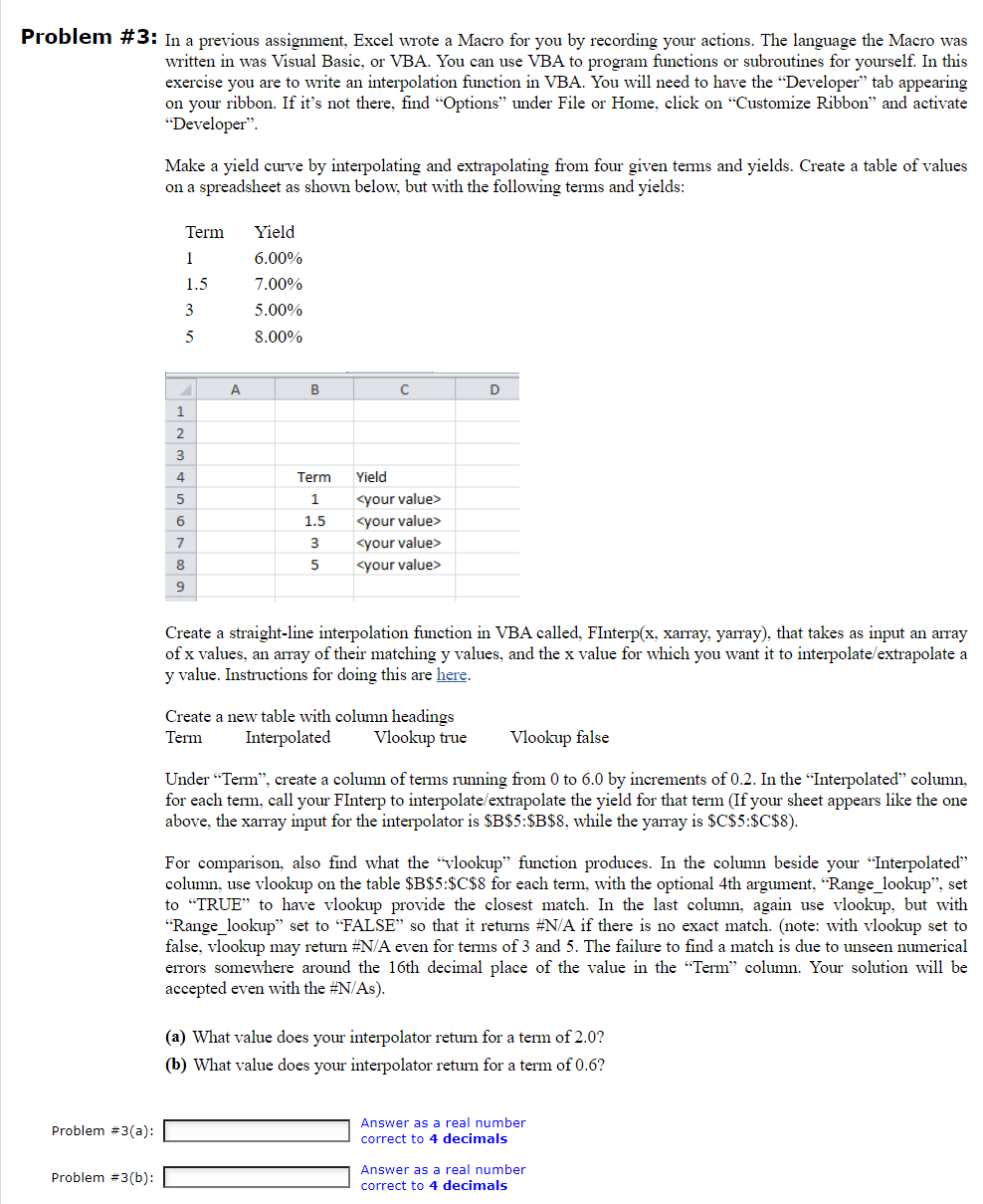
Problem #3: In a previous assignment, Excel wrote a Macro for you by recording your actions. The language the Macro was written in was Visual Basic, or VBA. You can use VBA to program functions or subroutines for yourself. In this exercise you are to write an interpolation function in VBA. You will need to have the Developer tab appearing on your ribbon. If it's not there, find "Options under File or Home, click on Customize Ribbon and activate "Developer" Make a yield curve by interpolating and extrapolating from four given terms and yields. Create a table of values on a spreadsheet as shown below, but with the following terms and yields: Term 1 Yield 6.00% 7.00% 5.00% 1.5 3 5 8.00% A B D 2 3 Hmino00 Term 1 5 6 1.5 Yield syour value> your value> your value> your value> 3 5 9 Create a straight-line interpolation function in VBA called, FInterp(x, xarray, yarray), that takes as input an array of x values, an array of their matching y values, and the x value for which you want it to interpolate/extrapolate a y value. Instructions for doing this are here. Create a new table with column headings Term Interpolated Vlookup true Vlookup false Under "Term, create a column of terms running from 0 to 6.0 by increments of 0.2. In the "Interpolated" column, for each term, call your FInterp to interpolate/extrapolate the yield for that term (If your sheet appears like the one above, the xarray input for the interpolator is $B$5:$B$8, while the yarray is $C$5:$C$8). For comparison, also find what the "vlookup" function produces. In the column beside your "Interpolated column, use vlookup on the table $B$5:$C$8 for each term, with the optional 4th argument, Range_lookup", set to "TRUE" to have vlookup provide the closest match. In the last column, again use vlookup, but with Range_lookup" set to "FALSE" so that it returns #N/A if there is no exact match. (note: with vlookup set to false, vlookup may return #N/A even for terms of 3 and 5. The failure to find a match is due to unseen numerical errors somewhere around the 16th decimal place of the value in the "Term column. Your solution will be accepted even with the #N/As). (a) What value does your interpolator return for a term of 2.0? (b) What value does your interpolator return for a term of 0.6? Problem #3(a): Answer as a real number correct to 4 decimals Problem #3(b): Answer as a real number correct to 4 decimals Problem #3: In a previous assignment, Excel wrote a Macro for you by recording your actions. The language the Macro was written in was Visual Basic, or VBA. You can use VBA to program functions or subroutines for yourself. In this exercise you are to write an interpolation function in VBA. You will need to have the Developer tab appearing on your ribbon. If it's not there, find "Options under File or Home, click on Customize Ribbon and activate "Developer" Make a yield curve by interpolating and extrapolating from four given terms and yields. Create a table of values on a spreadsheet as shown below, but with the following terms and yields: Term 1 Yield 6.00% 7.00% 5.00% 1.5 3 5 8.00% A B D 2 3 Hmino00 Term 1 5 6 1.5 Yield syour value> your value> your value> your value> 3 5 9 Create a straight-line interpolation function in VBA called, FInterp(x, xarray, yarray), that takes as input an array of x values, an array of their matching y values, and the x value for which you want it to interpolate/extrapolate a y value. Instructions for doing this are here. Create a new table with column headings Term Interpolated Vlookup true Vlookup false Under "Term, create a column of terms running from 0 to 6.0 by increments of 0.2. In the "Interpolated" column, for each term, call your FInterp to interpolate/extrapolate the yield for that term (If your sheet appears like the one above, the xarray input for the interpolator is $B$5:$B$8, while the yarray is $C$5:$C$8). For comparison, also find what the "vlookup" function produces. In the column beside your "Interpolated column, use vlookup on the table $B$5:$C$8 for each term, with the optional 4th argument, Range_lookup", set to "TRUE" to have vlookup provide the closest match. In the last column, again use vlookup, but with Range_lookup" set to "FALSE" so that it returns #N/A if there is no exact match. (note: with vlookup set to false, vlookup may return #N/A even for terms of 3 and 5. The failure to find a match is due to unseen numerical errors somewhere around the 16th decimal place of the value in the "Term column. Your solution will be accepted even with the #N/As). (a) What value does your interpolator return for a term of 2.0? (b) What value does your interpolator return for a term of 0.6? Problem #3(a): Answer as a real number correct to 4 decimals Problem #3(b): Answer as a real number correct to 4 decimals


